We propose a new CT perfusion analysis algorithm without deconvolution: Theoretically calculating the time-enhancement curve (TEC) under various perfusion conditions, finding a theoretical TEC that best fits the observed TEC, and using the theoretical TEC's perfusion parameters as the estimations for the observation point (FiTT).
The FiTT analysis procedure was as follows: First, the TEC of the arterial input function (AIF) was fitted to the gamma distribution function. Next, we defined the residual functions (R(t)s) that assume various perfusion states of brain tissue, and theoretical brain TECs were calculated by convolution of the AIF and R(t)s. Finally, we determined a theoretical TEC with the least error from the observed brain tissue TEC, using the theoretical TEC's perfusion parameters as the estimations for the observation point.
The estimation accuracy of FiTT was comparing an academic analyzer (bSVD algorithm) and a commercial analyzer (Bayesian algorithm) using a digital phantom. The verification items were visual evaluation of parametric maps, the relationship between ground truth and estimates, the effect of R(t) shape, the effect of AIF type, and the effect of source image noise.
Parametric map findings: For the academic analyzer, Tmax was affected by mean transit time (MTT); for the commercial analyzer, MTT was modulated by delay; for FiTT, CBV was slightly affected by MTT. The global characteristics and effect of the R(t) shape: The academic analyzer underestimated MTT, and tracer delay varied; the commercial analyzer had a positive bias for cerebral blood volume (CBV); and for FiTT, CBV and tracer delay estimated close to ground truth, cerebral blood flow (CBF) and MTT were affected by the R(t) shape. The effect of AIF type: The academic analyzer was independent; for the commercial analyzer, CBF, CBV, and tracer-delay were affected; for FiTT, CBF and CBV were affected. The effect of source image noise on parametric map noise: The academic analyzer was affected slightly; the commercial analyzer was unaffected; for FiTT, CBF map was affected. The effect of source image noise on the estimation bias: All analyzers were independent. The effect of the source image noise on the correlation coefficients (ground truth and estimates): None of the analyzers showed obvious proportional relationships.
The three analyzers were affected by one or more of noise, AIF type, and R(t) shape. Therefore, the estimates were overestimated, underestimated, biased, varied, and interacted. FiTT depended on R(t) shape and parametric map noise was affected by source image noise; however, estimates were close to ground truth and showed good linearity in many cases. Because clinical cases were not evaluated, the clinical behavior of FiTT is unknown. Within the scope of this study, we conclude that the estimation accuracy of FiTT is comparable to that of the academic and the commercial analyzer.
CT perfusion, Deconvolution, Quantitative imaging, Singular value decomposition, Stroke imaging, Bayesian estimation, Digital phantom
Knowing the size of the ischemic core and penumbra helps determine the appropriate endovascular treatment for acute stroke [1,2]. CT perfusion (CTP) can be performed following plain CT, and information on ischemic core size, penumbra size, cerebrovascular stenosis, occlusion, and collateral circulation can be obtained through a series of examinations, which have high clinical utility [3].
At present, the tracer-delay independent singular value decomposition (bSVD) method is widely used. However, because the solution oscillates with image noise, this method requires regularization. Several methods have been proposed for determining the regularization parameters, which are constant or case-specific values for each analyzer [4-6]. Therefore, when the size of the ischemic core or penumbra is to be measured, a threshold value must be set for each analyzer [7-9]. Various studies have been conducted to reduce source image noise and stabilize deconvolution [10-14].
In the 1990s, the rectangular model based "BOX-MTF" was put into clinical use [15]. Subsequently, Bennink, et al. presented a tracer-independent method of box NLR. The model-based approach is robust for scan truncation and sparse sampling because it can interpolate and extrapolate of the sampling points [16]. However, the perfusion parameters cannot be estimated accurately unless the analytical model and the subject's residual function match [17,18]. We assume that the gamma distribution function model is more physiological than the rectangular model. Here, we propose a new CTP analysis algorithm without deconvolution: Theoretically calculating the TEC under various perfusion conditions, finding a theoretical TEC that best fits the observed TEC, and using perfusion parameters of the theoretical TEC as estimates of the observation point (FiTT).
Analysis principle of FiTT: The time-concentration curve (TCC) of the indicator in brain tissue is calculated by the convolution of the input artery TCC and residue function (R(t)), scaled by blood flow (Equation 1). R(t) represents the brain tissue's blood flow character [19,20].
where, is the convolution operator, Ctss(t) is TCC of the brain tissue (g/ml), Cart(t) is the input artery TCC (g/ml), and F is blood flow (ml/s). In actual CTP, TCC is converted to Hounsfield units (HU) and observed as TEC.
The analysis procedure of FiTT was as follows: The input artery TEC was fitted to a gamma distribution function and converted to TCC. Next, we defined R(t)s for various perfusion conditions of brain tissue, modeled by the gamma distribution function. We then convolved the input artery TCC and R(t)s to obtain the theoretical TECs. Finally, we determined the theoretical TEC that best fit the observed TEC and used that theoretical TEC's perfusion parameters as the estimations for the observation point. Figure 1 shows the conceptual diagram.
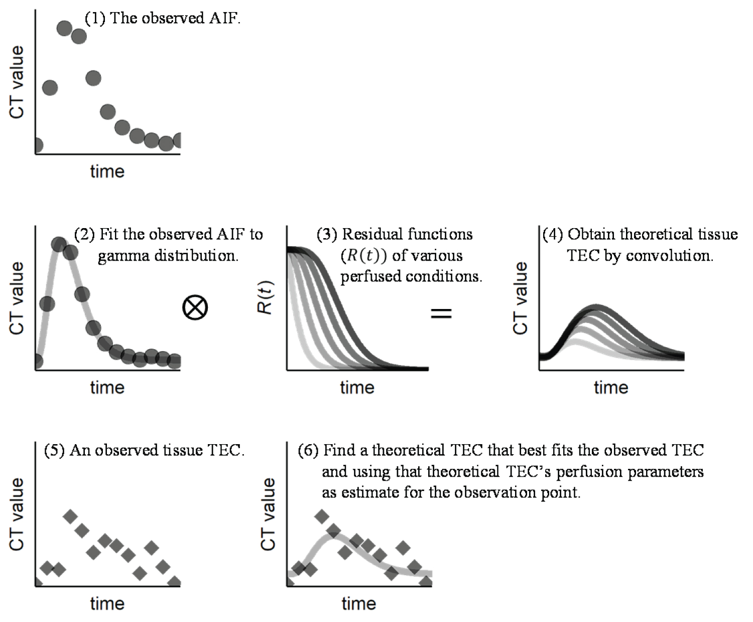 Figure 1: Conceptual diagram of analysis principle of FiTT.
AIF: Arterial Input Function; TEC: Time-Enhancement Curve.
View Figure 1
Estimation of AIF: The contrast medium was rapidly injected from the upper extremity vein, gradually diluted, and followed the gamma distribution in the internal carotid artery [21,22]. In the simulation study of CTP, we used an AIF modeled by Equation 2 that is used widely [7,16,17].
Where Cart(t) is the TCC of input artery, αart is the gamma distribution's shape parameter, and βart is the gamma distribution's scale parameter.
The TEC of the input artery (Eart(t)) observed in a dynamics can be expressed by k by adding a concentration-HU conversion factor (kHU), a CT value baseline (E0art), and a time offset (t0art) to Equation 2.
We used the nonlinear least-squares method to calculate each term in Equation 3.
Perfusion model: The gamma distribution function has the mathematical property of reproducibility, which means that the convolution of gamma distributions with the same scale parameter will result in the same distribution family [23,24]. Although the true R(t) of the brain has not been clarified [16,19], the indicator dilution curve observed in various regions of the human body can be explained by the gamma distribution. Therefore, we assumed that gamma distribution's reproducibility applied to the diluting process of brain tissue and used the gamma distribution function for the perfusion model of FiTT. The gamma distribution function was determined by the shape parameter, α, and the scale parameter, β. For simplicity, the scale parameter of the perfusion model is the same as the scale parameter of the AIF (βtss = βart).As the expected value of the gamma distribution function is α . β, mean transit time (MTT) can be expressed as:
and R(t) can be expressed as
where γ is the lower incomplete gamma function, Γ is the gamma function, and γ(α,t/β)Γ(α)-1 is the cumulative distribution function of the gamma distribution.
Theoretical TECs: The TEC of brain tissue Etss(t), observed in the dynamic scan, can be expressed by Equation 6 by adding a concentration-HU conversion factor kHU, a hematocrit correction factor kHT, a CT value baseline E0TSS, and a tracer delay (time offset from Eart(t))t0tss to Equation 2.
Note that E0tss is a variable in Equation 6. This allows us to estimate the baseline (i.e., the CT value before the introduction of the contrast medium).
In this study, kHU was set to 100, and kHt was set to a ratio of the large vessel (HLV = 0.45) to the small vessel (Hsv = 0.25) [25].
Blood flow F, was obtained from cerebral blood volume (CBV) and MTT using the central volume principle.
For the perfusion parameters of brain tissue, we defined that FiTT can be estimated for 1.5-2 times the normal or abnormal ranges and calculated 540582 theoretical TECs based on the above equations (Table 1). For the perfusion parameters of capillaries, we calculated 16775 theoretical TECs. Tissues that matched this template had each perfusion parameter set to zero during the vessel elimination process (Table 2).
Table 1: Parameters of the theoretical time-enhancement curves (TECs) for brain tissue.
There were 653310 combinations of each perfusion parameter, although combinations of high flow (CBF > 120 ml∙(100 g) ^ (-1)∙min ^ (-1)) and low flow (CBF < 5 ml∙(100 g) ^ (-1)∙min ^ (-1)) parameters were excluded, which resulted in 540582 theoretical TECs for brain tissue. View Table 1
Table 2: Parameters of the theoretical time-enhancement curves (TECs) for capillaries.
Parameters of the theoretical TECs for highly perfuse areas. If the TEC of a region matched this, the region was considered a vessel, and the estimates of each perfusion parameter were set to 0 during the vessel elimination process. A hematocrit correction factor of 1 was used. View Table 2
Estimation of perfusion parameters: The source images were down-sampled from 512 × 512 pixels to 256 × 256 pixels. A Gaussian filter (σ = 0.75) was applied to the source images to reduce noise. For each pixel, the sum of squared errors between the observed and the 557357 theoretical TECs was calculated to determine the theoretical TEC that had the least error. Perfusion parameters of the theoretical TEC were used as the estimated perfusion parameters of the pixel. If the estimated CBV was > 8 ml·100 g-1, it was considered a vessel [26], whereas if the estimated cerebral blood flow (CBF) was < 5 ml·100 g-1·min-1, it was considered as a non-perfuse region, and all estimates were set to 0.
Control analyzers: We compared the following two software to investigate the accuracy of FiTT: The bSVD method of PMA v5.0.5358.55864 (Kudo, et al. ASIST-Japan) [27], which is an academic research software (Acute Stroke Imaging Standardization Group, Japan). The accuracy of this software has been clinically and numerically verified, and compared with many analyzers [6,7,28,29]. This is no longer a publicly accessible software; and the Bayesian method in the Brain Perfusion 4D application of Vitrea v7.11.0.596 (Canon Medical Systems, Tochigi, Japan), a commercial general-purpose image processor. Both analyzers were used with default settings.
Digital phantom: We created a digital phantom with some extensions that faithfully reproduced the main characteristics of the phantom of Kudo, et al. [7]. The original phantom of Kudo, et al. consisted of patches with seven MTTs (24, 12, 8, 6, 4.8, 4, and 3.4s) and seven delays (0, 0.5, 1, 1.5, 2, 2.5, and 3s), placed on a human head CT. The artery, vein, five CBVs (1, 2, 3, 4, and 5 ml/100 g), and three R(t) shapes (exponential, linear, and box) were stacked in the slice direction. Gaussian noise was added to the image (signal-to-noise ratio = 5). The time phase was from 0 to 58 s in 2 s intervals. We added an R(t) shape, four AIF types, and six noise levels to the original phantom of Kudo, et al. (Figure 2 and Figure 3).
 Figure 2: In-plane configuration of the extended digital phantom.
The digital phantom based on a plain CT of the human head, which included patches, an artery and a vein that changed in intensity over time.
View Figure 2
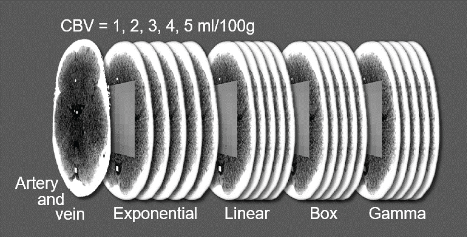 Figure 3: Slice direction configuration of the extended digital phantom.
The first slice had the artery and vein embedded, and subsequent slices had the patches embedded. The R(t) shapes of the patches were exponential, linear, box, and gamma distribution. Each R(t) shape contained patches with CBV = 1-5 ml/100 g.
View Figure 3
The additional R(t) shape had a gamma distribution (Equation 5) that perfectly matched the analysis model of FiTT. This gamma-distributed R(t) was used solely to check whether FiTT could be calculated accurately according to the algorithm. The above four R(t) shapes are shown in Figure 4.
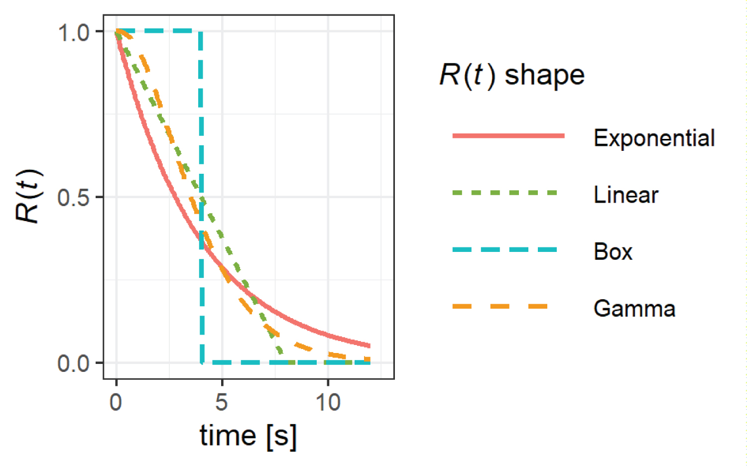 Figure 4: Example of the residual function R(t) of the extended digital phantom (MTT = 4s, CBV = 4 ml/100 g, β = 1.5).
View Figure 4
Figure 4: Example of the residual function R(t) of the extended digital phantom (MTT = 4s, CBV = 4 ml/100 g, β = 1.5).
View Figure 4
We defined the AIF of the phantom of Kudo, et al. as "standard" and added the following four AIFs based on the "standard" AIF:"A," decreased injection rate without changing injection volume; "B," increased injection rate without changing injection volume; "C," decreased injection volume by 30% and increased injection rate so that the maximum CT value equals the "standard" AIF; and "D", 1.5 times increase in injection volume (Figure 5 and Table 3).
Table 3: All the AIFs parameters in the extended digital phantom. MTTbolus is the MTT of the contrast bolus, which is the expected value of the gamma distribution function (α·β). Area under the curve (AUC) is proportional to the contrast dose. View Table 3
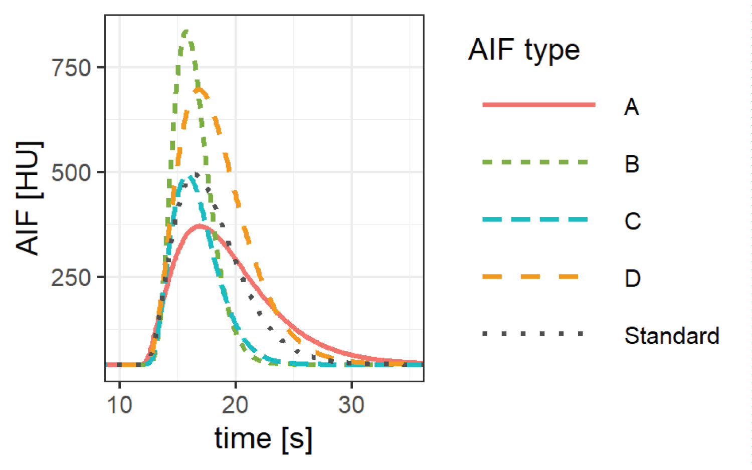 Figure 5: All the AIFs in the extended digital phantom.
View Figure 5
Figure 5: All the AIFs in the extended digital phantom.
View Figure 5
To investigate the effect of noise, we created datasets with Gaussian noise (standard deviation of 0 to 15 in intervals of 2.5). The noise level of the phantom of Kudo, et al. was determined using the average clinical CTP, which has a signal-to-noise ratio of 5; this was approximately 7.2 standard deviations. The standard noise level of the extended digital phantom was set to 7.5. The commercial analyzer showed a strong smoothing process in the z-direction. To reduce the effect of smoothing, five slices of patches with the same intensity and noise were stacked. The parametric image of the central slice (the third slice) was used for data analysis.
A CT image of a human head was downloaded from the DICOM Library [30]. The head CT image was deformed to place patches in the skull. With other minor changes, the phantom of Kudo, et al. had an artery and vein embedded only in the first slice, whereas our extended phantom had them embedded in all slices.
We created CBF, CBV, MTT, and tracer delay maps for all the analyzers. For quantitative evaluation, a 28 × 28-pixelregion of interest was placed in the center of each patch. The mean value of the region of interest was used as the estimation value of the perfusion parameter, and the standard deviation was used as the noise of the perfusion parameter.
As the tracer delay parameter, the academic analyzer outputs "Tmax" and the commercial analyzer and FiTT output "Delay." In this study, we consider "Tmax" and "Delay" to be equivalent and use the term "Tracer delay" [31]. We excluded MTT = 24 s (leftmost column of the patches embedded for the extended digital phantom) for all analyzers' quantitative evaluations. This was because FiTT is not able to estimate MTTs > 15 s. We also excluded the gamma-distributed R(t) in the analyzer comparison experiments. This was to avoid bias in favor of FiTT because the gamma-distributed R(t) was in perfect agreement with the FiTT analytical model.
The correlation between the ground truth and each perfusion parameter's estimates was determined using Pearson's correlation coefficient and linear regression. We set r > 0.9 to represent a strong correlation. In the investigation of the effect of the R(t) shape, differences between the estimates for each R(t) shape were tested by analysis of covariance (ANCOVA) and Turkey's multiple comparisons. In the investigation of the effect of the AIF type, similar tests were performed for each AIF type. Estimation bias was calculated using the following equation:
To ensure that FiTT can estimate the perfusion parameters as designed, we estimated for a portion of the extended digital phantom (noise = 0, gamma-distributed R(t), standard AIF). Figure 6 shows the relationship between the ground truth and the estimates. The CBF pulsated slightly, but all perfusion parameters were in good agreement. The correlation coefficient was close to 1, the slope of the linear regression was close to 1, and its intercept was close to 0 (Table 4). FiTT conformed to the analysis principle.
Table 4: The correlation coefficients and regression equations between the ground truth and perfusion parameter estimates for FiTT. The R(t) shape was the gamma distribution, AIF was the standard type, and the source image noise had a standard deviation of zero. Those marked with * are ρ > 0.9, which was considered a strong correlation. View Table 4
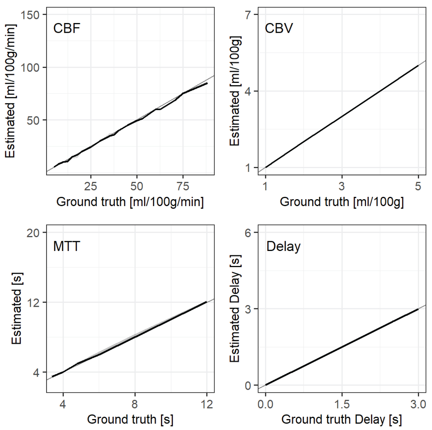 Figure 6: The relationship between the ground truth and the perfusion parameter estimates for FiTT. The R(t) shape is the gamma distribution, AIF is the standard type, source image noise has a standard deviation of 0. Solid lines represent the medians of the estimates. Shaded areas represent the interquartile ranges (IQR), and the gray solid lines are y = x.
View Figure 6
Figure 6: The relationship between the ground truth and the perfusion parameter estimates for FiTT. The R(t) shape is the gamma distribution, AIF is the standard type, source image noise has a standard deviation of 0. Solid lines represent the medians of the estimates. Shaded areas represent the interquartile ranges (IQR), and the gray solid lines are y = x.
View Figure 6
Examples of parametric maps are shown in Figure 7. The tracer delay of the academic analyzer was affected by MTT. MTT of the commercial analyzer was modulated by delay. FiTT was slightly affected by MTT for CBV, and it was inaccurate for MTT = 24 s (leftmost column of the patches) because MTT could only be measured up to 15 s.
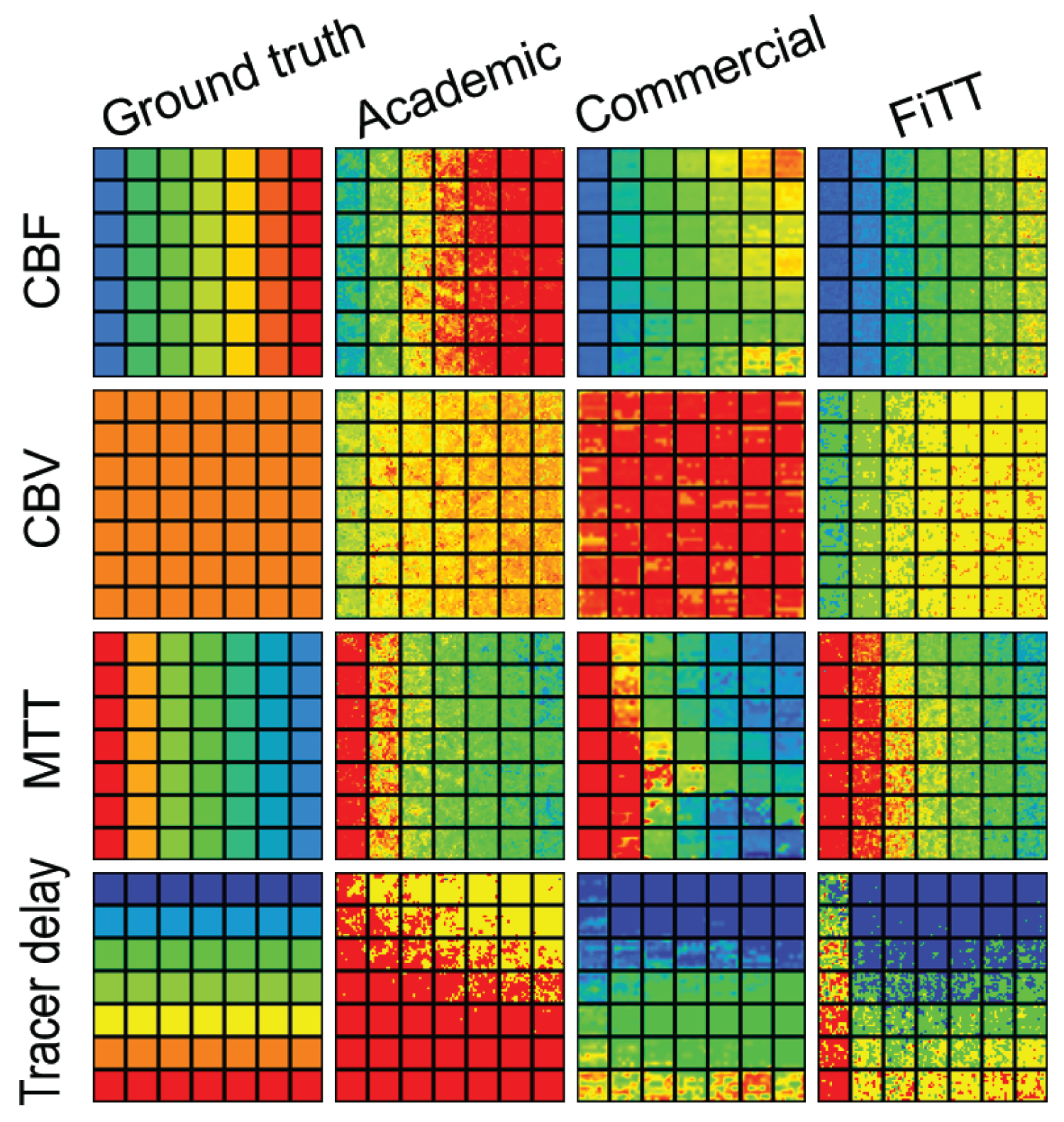 Figure 7: Examples of parametric maps. AIF was the standard type, source image noise was at the standard level, CBV = 5 ml/100 g, and R(t) shape was exponential. The horizontal direction of the map is MTT (24 to 3.4 s, left to right) and the vertical direction is tracer delay (0 to 3 s, top to bottom).
View Figure 7
Figure 7: Examples of parametric maps. AIF was the standard type, source image noise was at the standard level, CBV = 5 ml/100 g, and R(t) shape was exponential. The horizontal direction of the map is MTT (24 to 3.4 s, left to right) and the vertical direction is tracer delay (0 to 3 s, top to bottom).
View Figure 7
Figure 8 shows the relationship between the ground truth and estimates of each R(t) shape. The ANCOVA showed that the CBV of the commercial analyzer was not significant (p = 0.07), whereas all others were significant (p < 0.01).
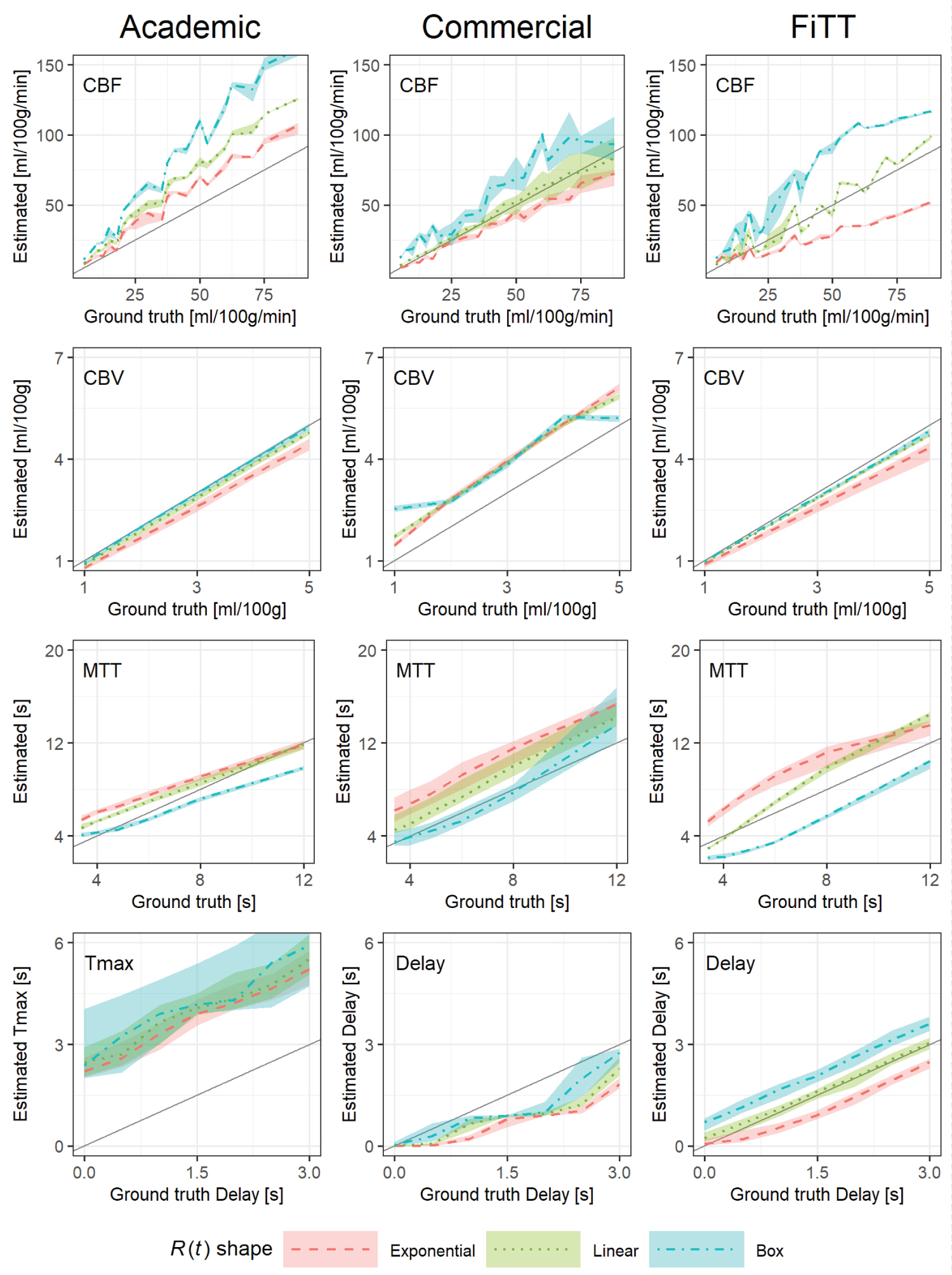 Figure 8: The relationship between the ground truth and estimates for each R (t) shape. AIF was the standard type; source image noise was at the standard level. The various dashed lines are the medians of each R(t) shape. The shaded areas represent the interquartile ranges, and the gray solid line is y = x.
View Figure 8
Figure 8: The relationship between the ground truth and estimates for each R (t) shape. AIF was the standard type; source image noise was at the standard level. The various dashed lines are the medians of each R(t) shape. The shaded areas represent the interquartile ranges, and the gray solid line is y = x.
View Figure 8
The trends common to all analyzers were as follows: CBV had little variation; CBF, MTT, and tracer delay were affected by R(t) shape; for MTT, exponential R(t) was overestimated, and boxed R(t) was underestimated, and vice versa for CBF and the linear R(t) was similar across perfusion parameters.
The characteristics of each analyzer were as follows: The academic analyzer underestimated MTT (the slope of the linear regression for a mixture of R(t) was 0.74) and consequently overestimated CBF, tracer delay showed large variation, and correlation coefficients were low (0.54-0.76); the commercial analyzer had a positive bias for CBV (the linear regression intercept for a mixture of R(t) was 0.991 ml·100 g-1); For CBF of FiTT, the correlation coefficients of each R(t) shape was strong, and those linear regression slopes varied (0.5-1.46), although the correlation coefficients for a mixture of R(t) was decreased (0.75), MTT had the same tendency; For CBV and tracer delay of FiTT, estimates were close to ground truth and had excellent linearity. See #1 and #2 of the Supplimentary File for details about the correlation coefficients, regression equations, and results of Turkey's multiple comparisons.
The five AIF types were examined for their effects on estimates. Figure 9 shows the relationship between the ground truth and estimates for each AIF type (see #3-7 of the Supplimentary File for figures). The ANCOVA for the AIF type was p < 0.02 for all perfusion parameters.
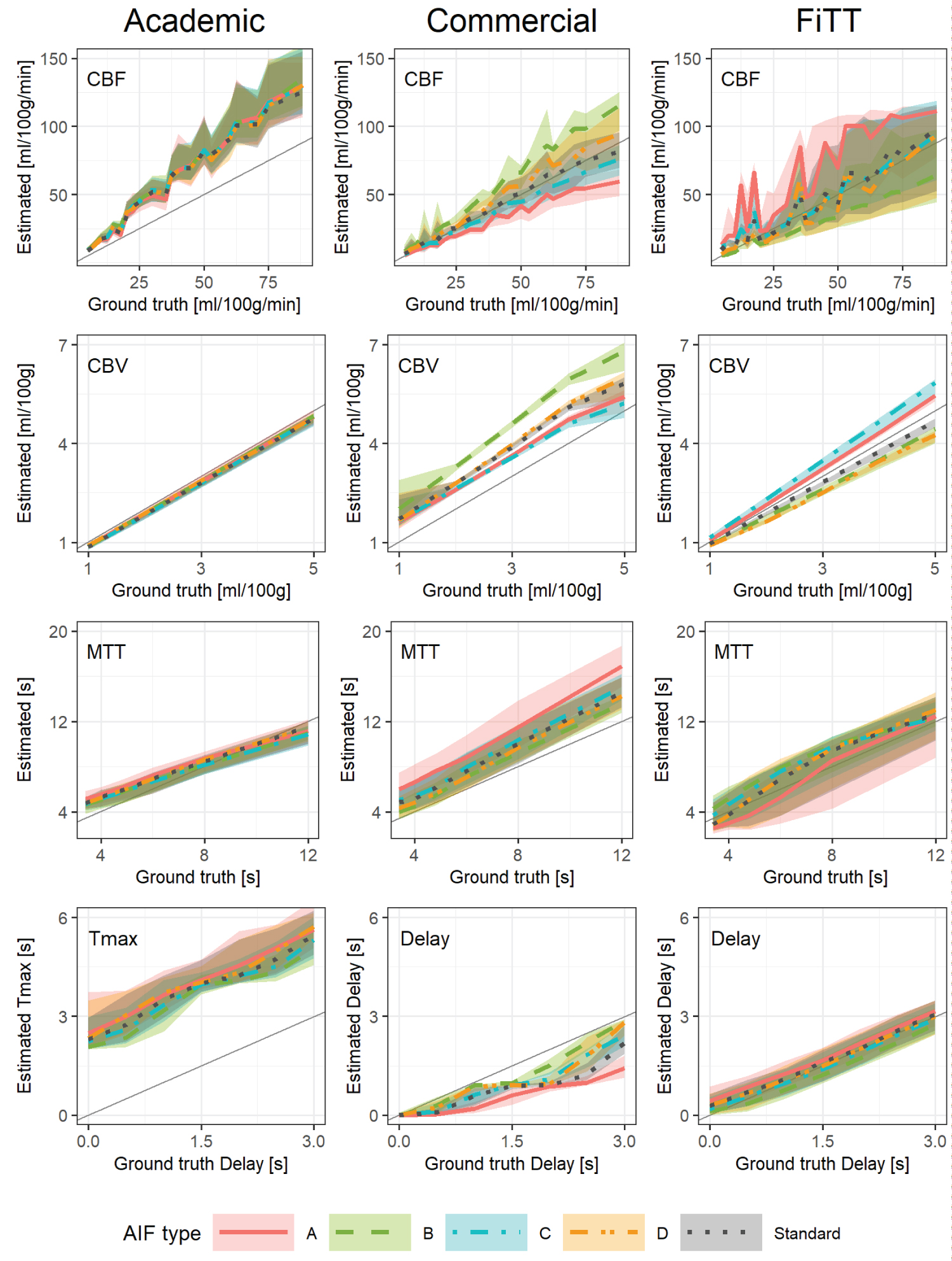 Figure 9: The relationship between the ground truth and estimates of perfusion parameters for each AIF type. "Standard," the AIF of the phantom of Kudo, et al. "A," decreased injection rate without changing injection volume; "B," increased injection rate without changing injection maximum CT value equals the "standard" AIF; "C," decreased injection volume by 30% and increased injection rate so that the maximum CT value equals the "standard" AIF; and "D," 1.5 times increase in injection volume. The source image noise was at the standard level; and R(t) shape was a mixture of exponential, linear, and box. Lines are the medians, shaded areas are interquartile ranges, and gray solid lines represent y = x.
View Figure 9
Figure 9: The relationship between the ground truth and estimates of perfusion parameters for each AIF type. "Standard," the AIF of the phantom of Kudo, et al. "A," decreased injection rate without changing injection volume; "B," increased injection rate without changing injection maximum CT value equals the "standard" AIF; "C," decreased injection volume by 30% and increased injection rate so that the maximum CT value equals the "standard" AIF; and "D," 1.5 times increase in injection volume. The source image noise was at the standard level; and R(t) shape was a mixture of exponential, linear, and box. Lines are the medians, shaded areas are interquartile ranges, and gray solid lines represent y = x.
View Figure 9
The academic analyzer was independent, but the tracer delay showed considerable variability (the correlation coefficient was 0.63-0.71). The commercial analyzer was affected for CBF, CBV and tracer delay. FiTT was affected for both CBF and CBV. For "A" the low CBF region was particularly overestimated. The linear and box shape R(t) were also overestimated (not represented in figures).For most of the perfusion parameter estimates for all analyzers, "standard" and "D" were close together, and "A" and "B" were divergent. See #8 and #9 of the Supplimentary File for details about the correlation coefficients, regression equations, and Turkey's multiple comparison results.
Figure 10 shows the relationship between source image noise and parametric map noise.
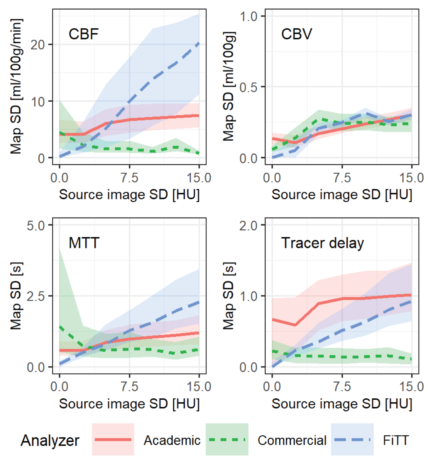 Figure 10: Relationship between source image noise and parametric map noise. The lines represent the medians of parametric map noise, and the shaded areas are interquartile ranges. AIF type was "standard" and the R(t) shape was a mixture of exponential, linear, and box.
View Figure 10
Figure 10: Relationship between source image noise and parametric map noise. The lines represent the medians of parametric map noise, and the shaded areas are interquartile ranges. AIF type was "standard" and the R(t) shape was a mixture of exponential, linear, and box.
View Figure 10
When the standard deviation of source image noise was > 0.25, the academic analyzer's parametric map noise was affected slightly, whereas the commercial analyzer was almost unaffected. FiTT was more strongly affected than the other analyzers, especially for CBF.
Figure 11 shows the relationship between source image noise and estimation bias. Overall, each analyzer had a constant estimation bias that was independent. The academic analyzer had a large estimation bias for tracer delay.
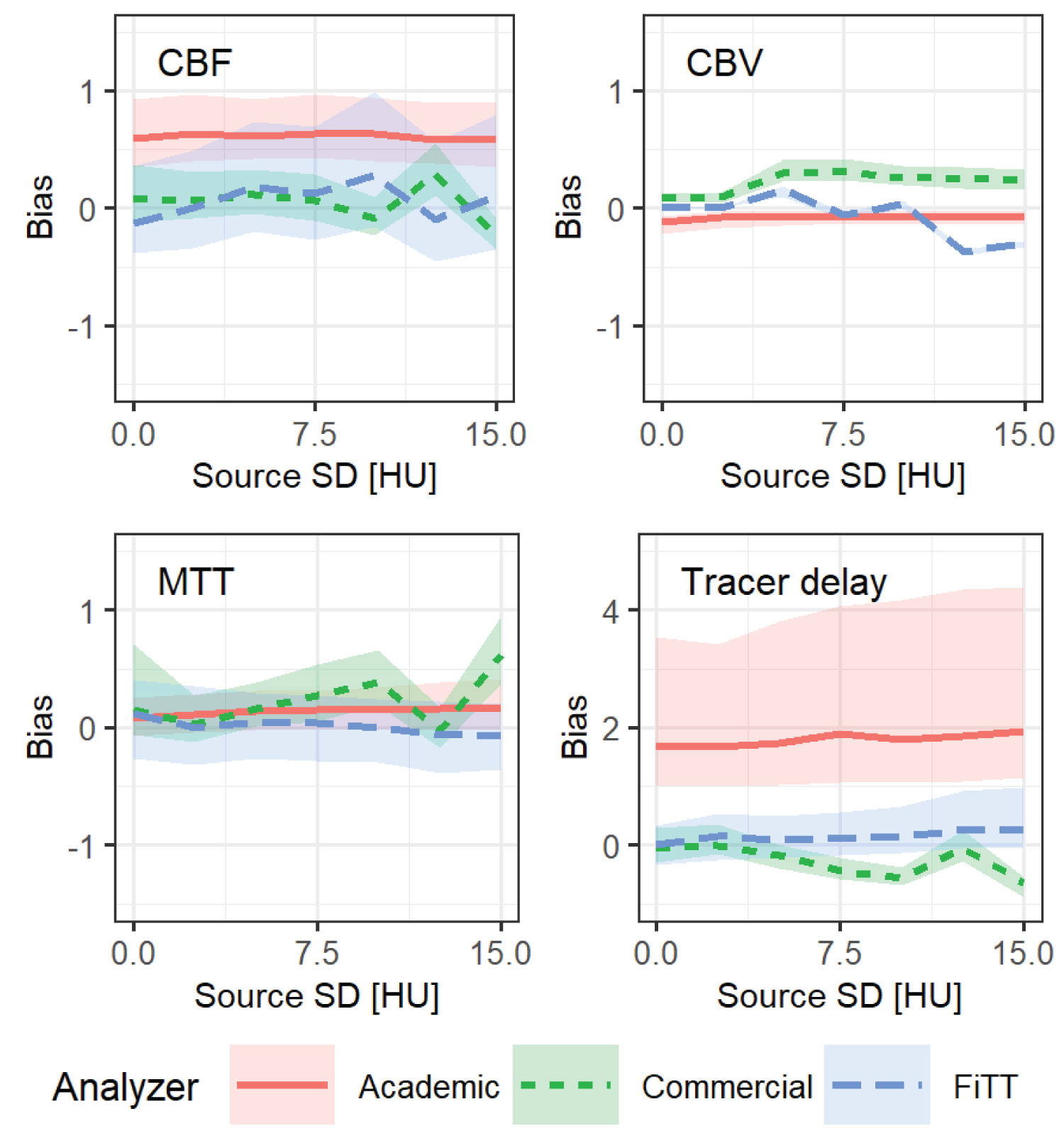 Figure 11: Relationship between source image noise and estimation bias. The lines represent medians of estimation bias, and shaded areas are interquartile ranges. AIF type was "standard" and the R(t) shape was a mixture of exponential, linear and box.
View Figure 11
Figure 11: Relationship between source image noise and estimation bias. The lines represent medians of estimation bias, and shaded areas are interquartile ranges. AIF type was "standard" and the R(t) shape was a mixture of exponential, linear and box.
View Figure 11
Figure 12 shows the relationship between source image noise and correlation coefficients (ground truth and estimates). For each perfusion parameter, the graph lines were slightly sloped or fluctuated erratically, and there was no obvious proportional relationship between source image noise and the correlation coefficient. For tracer delay of the academic analyzer, the correlation coefficient was low and fluctuated. For the commercial analyzer, the correlation coefficient was low when the source image noise was favorable (i.e., < 5). For FiTT, the correlation coefficient was low when the source image noise was > 10, except for that of CBV.
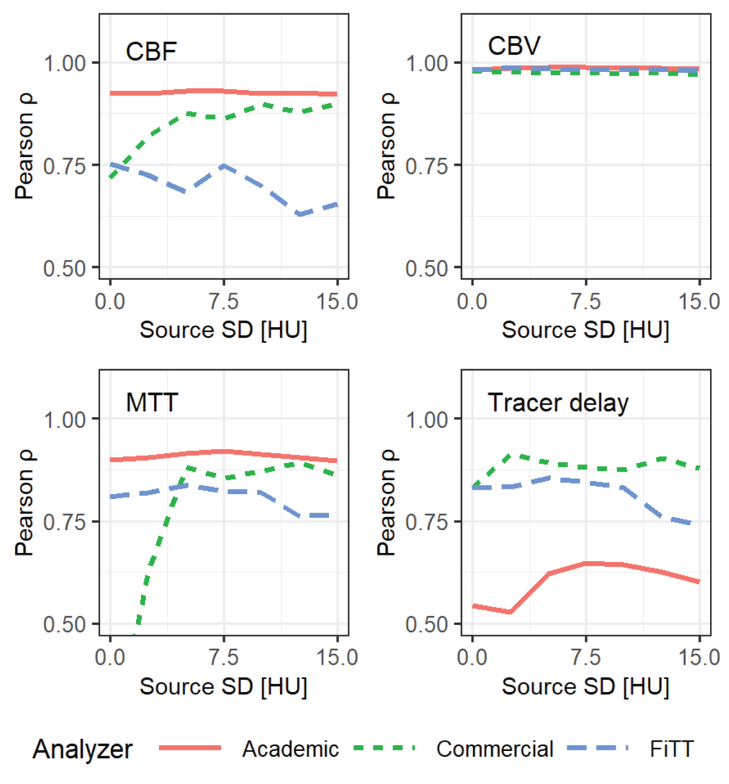 Figure 12: Relationship between source image noise (standard deviation (SD)) and Pearson's correlation coefficient (ground truth and estimates of perfusion parameters). AIF type was "standard" and the R(t) shape was a mixture of exponential, linear and box.
View Figure 12
Figure 12: Relationship between source image noise (standard deviation (SD)) and Pearson's correlation coefficient (ground truth and estimates of perfusion parameters). AIF type was "standard" and the R(t) shape was a mixture of exponential, linear and box.
View Figure 12
Each analyzer was affected by one or more of noise, AIF type, and R(t) shape. As a result, the estimates were overestimated, underestimated, biased, and varied and there were interactions among perfusion parameters. FiTT was also more or less affected by these factors, and the estimates varied. However, the variation was less than that of the other analyzers. The estimates were also close to the ground truth and showed good linearity. Therefore, the estimation accuracy of FiTT in the numerical comparison tests was considered comparable with the academic and the commercial analyzer.
FiTT was affected by the R(t) shape for CBF and MTT. For each R(t) shape in CBF and MTT, the correlation coefficients were strong. The linear regression slopes were varied, but the correlation coefficient for a mixture of R(t) was decreased. This phenomenon indicates dependence on the R(t) shape. Because FiTT is a model-based analysis, the estimation accuracy cannot be avoided when the analytical perfusion model and the R(t) of the sample do not match [16-18].
For FiTT,"A" overestimated CBF, particularly when CBF was low. Although not shown in the results, the linear and boxed R(t) overestimated, and the exponential and gamma-distributed R(t) were nearly accurate. "A" had the lowest peak CT value compared with the other AIFs, which could reduce accuracy because of the smaller difference between each theoretical TEC. We believe the overestimation of CBF was mainly due to the decreased AIF enhancement. The effect on R(t) also worked in the same situation. FiTT estimated the AIF of the "standard" and "C" equally well. This suggests that the contrast agent can be reduced if the peak CT value is maintained around the "standard" type.
For FiTT, the parametric map noise increased with increased source image noise. The correlation coefficient and estimation bias were slightly affected. Thus, the estimation accuracy can be expected to persist even with high levels of noise. However, the noise limits cannot be determined without quantitative and qualitative evaluations of the clinical images such as those performed in various low-dose CTP studies [32-34]. We could not confirm acceptable noise limits because clinical images were not evaluated in the present study.
In this study, we could not evaluate the clinical images because of research limitations. Thus, FiTT is not yet ready for clinical use. Initially, it will be essential to verify the FiTT response to the contrast conditions, artifacts, beam hardening, and various tube voltages and verify whether the analytical model of FiTT is consistent with brain tissue R(t). This must be determined by numerous clinical cases. Patient and series selection; time and space sorting; automatic setting of AIF and venous output functions; saving of parametric maps; and connections with picture archiving and communication systems are all yet to be implemented.
FiTT takes a long time to calculate the square error between the large number of theoretical TECs and the observed TEC. FiTT took 18 minutes to calculate the single-slice 30-phase data using an old computer, whereas the academic analyzer took only 10 seconds. Coarse sampling of theoretical TECs would speed up this process. FiTT was built on R, a free software environment for statistical computing and graphics [35]. R is relatively fast among interpreted languages but its implementation in a compiler language or using parallel processing would further reduce the computation time.
We have proposed FiTT as a new CTP analysis algorithm without deconvolution. The effects of R(t) shape, AIF type, and source image noise on estimates were investigated using a digital phantom. We conclude that the estimation accuracy of FiTT is comparable to that of academic and commercial analyzers in numerical simulation studies.
The authors have no conflicts of interest to disclose.
HI conceived of the presented idea; developed the theory; performed the simulation and the analysis; and wrote the paper. AS and HI validated experiments and results. AS supervised the findings of this work. All authors discussed the results and contributed to the final manuscript.
None.