Substitution rate matrices are used to correct multiple hits at the same sites, which requires the derivation of transition probabilities and evolutionary distances from substitution rate matrices. The derivation is essential in molecular phylogenetics and phylogenomics, and represents the only statistically sound way for developing scoring matrices used in sequence alignment and local string matching (e.g., BLAST and FASTA). Three different approaches are frequently used for deriving transition probabilities and evolutionary distances: 1) The probability reasoning, 2) Solving partial differential equations, and 3) Matrix exponential and logarithm. The first approach demands the least amount of mathematical skills but offers the best way for conceptual understanding, and can often generate nice mathematical expressions of transition probabilities and evolutionary distances. This review represents the most systematic and comprehensive numerical illustration of the first approach.
Substitution model, Substitution rate, Transition probability, Evolutionary distance
Substitutions occur over time and can overwrite each other at the same nucleotide or amino acid site. When we compare two homologous nucleotide sequences and find differences in N sites, the actual number of substitutions (designated by M) could be much greater than N because multiple substitutions could have happened at the same site, overwriting each other. Substitution models are used to infer the observable M from the observed substitutions from sequence comparisons.
Many substitution models have been proposed for nucleotide, amino acid and codon sequences. All substitution models used in molecular phylogenetics are Markov chain models characterized by 1) Either a transition probability matrix (P) with discrete time or a rate matrix (Q) in continuous time where P can be derived from Q, and 2) Equilibrium frequencies. The general form of an instantaneous rate matrix for nucleotide sequences is, in the order of A, G, C, and T:
Transition probability matrix, often referred to as the P matrix, specifies the probability of a nucleotide or amino acid changing into another one after time t. It is needed to calculate likelihood and to derive evolutionary distances, and consequently is needed phylogenetics based on the maximum likelihood and distance-based methods as well as Bayesian inference. Whether a substitution model can be implemented for phylogenetic analysis essentially depends on whether the model’s transition probabilities can be calculated.
There are three ways to obtain transition probabilities from the Q matrix [1,2] :1) By probability reasoning, 2) By solving differential equations involving rates, and 3) By taking the matrix exponential of the rate matrix. The last two require some mathematical background in calculus and linear algebra. The first, in contrast, demands little mathematical skill except for careful book-keeping and solving simultaneous equations. This approach is particularly relevant to biological students not only for gaining a conceptual understanding of the substitution models, but also to deriving nice mathematical expressions for transition probabilities and evolutionary distances. New researchers often ask why we can derive evolutionary distances between two aligned sequences for the TN93 model [3] but cannot for the simpler HKY85 model [4] which is a special case of the TN93 model, yet another model, F84 (used in PHYLIP since 1984), which is also a special case of the TN93 model, can have its evolutionary distance readily derived. One can easily obtain answers to such questions by taking the first approach. However, the first approach is not of general purpose and cannot handle very complicated substitution models. In contrast, the last one can be used with any substitution models specified by a rate matrix from which the matrix exponential can be obtained. In short, all these approaches need to be learned by anyone wishing to become a molecular phylogeneticist, but this paper will focus only on the probability reasoning approach illustrated with JC69 [5], K80 [6], F84 (the model used in PHYLIP since 1984), HKY85 [4], and TN93 [3] models.
Felsenstein [1] presented nice examples of probability reasoning to derive transition probabilities and evolutionary distances from rate matrices. This section presents the approach in a more systematic and accessible way.
Consider nucleotide A in the JC69 model (Figure 1a). Imagine that the nucleotide has a rate α of changing into any of the four nucleotides, i.e., including changing to itself (Figure 1b). This is effectively the same specification as the JC69 model. After time t, the expected number of substitutions is 4αt and the probability of no substitution is p (x = 0, α, t) = e-4αt according to the Poisson distribution, and the probability of having at least one change is then p (x ≥ 1, α, t) = 1-e-4αt (Figure 1c). Because nucleotide A can change into any one of the four nucleotides (including nucleotide A itself), each nucleotide gets 1/4 of p (x ≥ 1, α, t). We therefore have in Figure 1.
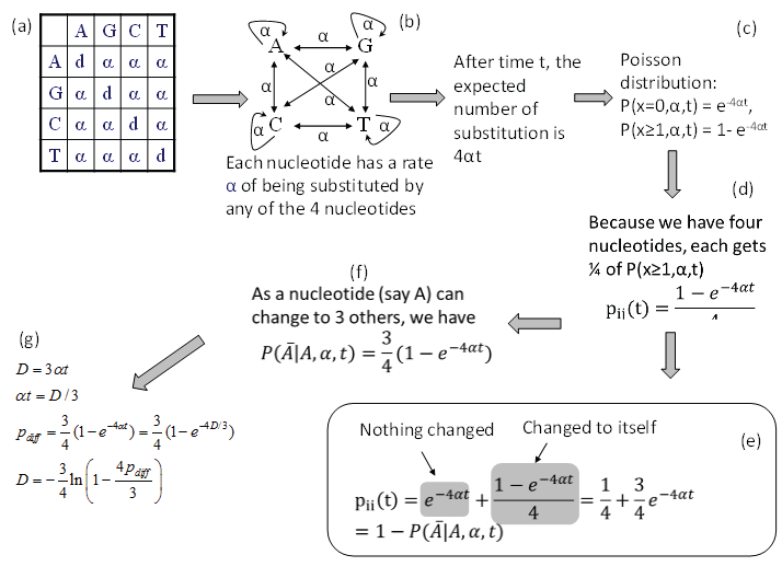 Figure 1: Derivation of transition probabilities and the evolutionary distance (D) based on the JC69 model. The d value in the diagonal of the rate matrix (a) is constrained by the row sum equal to 0, i.e., d = -3α. P(j|i,t) means the probability of changing from the original nucleotide i to nucleotide j after time t, and is synonymous to pij(t) or simply pij in this paper. View Figure 1
The transition probability pii(t) is the summation of two probabilities: the probability of no change (which is e 4αt) and the probability of changing to itself which is the same as specified in Eq. (2), as shown in Figure 1e, i.e.,
The transition probability matrix for the JC69 model has only two distinct elements. The four diagonal elements are the same as specified in Eq. (3) and all the off-diagonal elements are the same as specified in Eq. (2). Each row in P adds up to 1 as a nucleotide can either stay the same or change into some other nucleotides.
There are some quick ways to check the derived transition probabilities. First, we note that when t approaches infinity, then all entries in matrix P approaches ¼ if α > 0. This is what we have expected. Second, when t = 0, then all diagonal elements in matrix P are 1 and all off-diagonal elements are zero. This is again what we expected. Third, if α is zero, then no change is possible, and we again expect all diagonal elements in matrix P to be 1 and all off-diagonal elements to be zero, which is also true.
From pij in Eq. (2), the expected proportion of sites that are different between two aligned homologous sequences (pdiff) is 3*pij(t), i.e.,
Note that pdiff approaches ¾ when t is infinitely large, which means that multiple substitutions can no longer be corrected. Eq. (4) offers another way of deriving pii(t) in Eq. (3), i.e., pii(t) is simply 1-pdiff.
Eq. (4) allows us to derive the JC69 distance (DJC69) because a distance is defined as μt where μ is the substitution rate which is equal to 3α in the JC69 model. This is the same as the distance that you have driven is the product of the speed (rate) and time. Given that DJC69 = 3αt, we can derive DJC69 (Figure 1g) by substituting αt = DJC69/3 into Eq. (4), i.e.,
Where pdiff (the expected number of sites that are different between the two homologous sequences) can be approximated by the observed proportion of sites (pdiff.obs) differing between the two aligned sequences. Note that pdiff.obs may differ from pdiff even when the underlying substitution model indeed follows JC69 because of 1) Stochastic factors due to limited aligned length of the two sequences, and 2) Distortion caused by suboptimal sequence alignment. Thus, although pdiff in Eq. (4) cannot be greater than 0.75, pdiff.obs could, even when sequences evolve strictly according to the JC69 model. DJC69 is not defined when pdiff ≥ 0.75 as there is no logarithm for 0 or negative values.
We can optionally show that DJC69 in Eq. (5) is a maximum likelihood distance. For two aligned sequences of length N, designate the number of sites that differ between the two sequences as ND and the number of sites identical between the two sites as (N-ND). Now the likelihood function is:
Where the constant term N*ln(1/4) can be dropped in maximizing lnL to obtain the distance estimate, but needs to be kept when performing likelihood ratio test for comparing different substitution models (e.g., JC69 against TN93).
We take the derivative of lnL with respect to DJC69, set the derivative to 0 and solve for DJC69. The resulting DJC69 is exactly the same as that in Eq. (5). I used D instead of DJC69 in the equations below:
The variance of DJC69 (designated as VJC69) is obtained as the negative reciprocal of the second derivative of lnL:
Note that VJC69 decreases with sequence length L as one would have expected. We illustrate the application of Eqs. (5) and (8) by using the aligned sequences in Figure 2 where N = 24, ND = 6, and pdiff = 6/24 = 0.25. So DJC69 = 0.3041, and var (DJC69) = 0.0176.
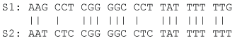 Figure 2: Two homologous sequences for illustrating computation of pairwise evolutionary distances. View Figure 2
The equilibrium frequencies of the π vector can be derived by set t = ∞ in Eqs. (2) and (3) which leads to pii = pij = ¼. This implies that equilibrium frequencies of the four nucleotides will be equal for the JC69 model. This is not surprising because the frequencies did not even appear in the rate matrix (Figure 1a).
The K80 model has a transition substitution rate α and a transversion rate β (Figure 3a). We will focus on nucleotide A and conceptualize the model with two events (Figure 3b), in contrast to only one event in the JC69 model. The first event (e1) occurs when nucleotide A changes into any of the four nucleotides (including to itself). In other words, the original A is replace by a nucleotide randomly drawn from a nucleotide pool with equal nucleotide frequencies. This event occurs with a rate β. The second event (e2) occurs when nucleotide A changes either to G or to itself, i.e., the original A is replace by a nucleotide randomly drawn from a purine pool with equal number of A and G. This e2 occurs with a rate γ. Thus the transition rate α equals β+γ according to this conceptualization. Note that, whenever e1 happens, the original nucleotide is replace by any one of the four nucleotides with equal probability, no matter how many e2 events has occur before or after the occurrence of e1. It might help to think of a long sequence with L sites being A at time 0. If these L sites each have experienced at least one e2 event, then these sites will either be A or G with equal probability (i.e., 0.5), and we expect to have L/2 sites being A and the other L/2 sites being G. In contrast, if each of these L sites has experienced at least one e1 event, then the site will be replaced by either A, C, G, or T with equal probability, and we expect to observe A, C, G and T in L/4 sites each. Any e2 events occurring before or after the e1 event do not change this expectation. This means that e1 erases e2, but not vice versa. The probability that an e2 event happened is informative only when no e1 event has happened.
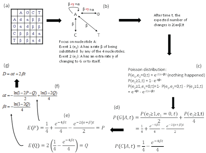 Figure 3: Derivation of transition probabilities and the evolutionary distance (D) based on the K80 model. The rate matrix (a) has the diagonal elements (d) constrained by the row sum equal to 0, i.e., d = -α - 2β. P and Q are the observed proportion of transitional and transversional changes between two aligned homologous sequences. Equating them to their respective expected values, E(P) and E(Q), leads to the solution of αt and βt shown, and the evolutionary distance D. P(j|i,t) means the probability of changing from the original nucleotide i to nucleotide j after time t, and is synonymous to pij(t) or simply pij in this paper. View Figure 3
After time t, the expected number of substitutions is 2(α+β)t, i.e., the nucleotide A has two ways of change with a rate of α (to A and to G) and another two ways of change with a rate β (to C and to T), so the probability of no change, according to Poisson distribution, is
Note that α is conceptualized as (β+γ) in Figure 3, so e-2(α+β)t in Eq. (9) is equivalent to e-(4β+2γ)t. The probability that at least one e1 event has occurred is
Thus, the probability that at least one e2 has occurred but e1 has not occurred is simply
These probabilities are also shown in Figure 3c. The reason for the condition that “e1 has not occurred” is because e1 event can erase e2 event (as we have discussed before).
Now the probability of the starting nucleotide A changing to G during time t, designated as p(G|A,t), is the summation of two probabilities. The first is 1/2 of the probability of p(e2 > 0, e1 = 0,t) in Eq. (11) because the other 1/2 is for A to itself. The second is 1/4 of p(e1 > 0,t) in Eq. (10) because A→A, A→G, A→C and A→T each get ¼, so only 1/4 of p(e1 > 0,t) is for A→G. The summation of these two probabilities (Figure 3d) is p(G|A,t). This probability is equal to p(A|G,t), p(C|T,t), and p(T|C,t) in the K80 model. In other words, the summation of these two probabilities is the probability of a transition (Ps) during time t. Thus,
Similarly, the probability of the starting A changing to C (or to T) is 1/4 of p(e1 > 0,t) in Eq. (10) because 1/4 is for A→A, ¼ is for A→G and 1/4 is for A→T, so only 1/4 is for A→C (Figure 3d). This probability is the probability for a transversional change during time t,
As a quick check of the derived transition probabilities, we note that Ps and Pv are zero when t = 0 (or when α = 0 and β = 0). This also implies that all diagonal elements in the transition probability matrix are equal to 1, and is what we have expected. When t = ∞, with α > 0 and β > 0, all entries in matrix P approaches ¼ (the equilibrium frequency of the K80 model). This is also what we expected.
For two aligned homologous sequences, Ps can be approximated by the proportion of sites differing by a transition (P), and 2Pv by the portion of sites differing by a transversion (Q, Figure 3e). Note that the expected Q is equal to 2Pv because there are two ways of having a transversional change. Therefore,
We can now first solve for βt from Eq. (15), and then substitute the solution for βt into Eq. (14) to solve for αt. This leads to
Recall that evolutionary distance is defined as μt, where μ is the substitution rate which is equal to (α+2β) in the K80 model. Thus, the evolutionary distance based on the K80 model (DK80) is (α+2β)t, which comes to
Where P and Q can be approximated by the observed proportion of sites differing by a transition or a transversion from two aligned sequences, designated as Pobs and Qobs. Similar to what I have mentioned with reference to DJC69, P and Q may differ from Pobs and Qobs even if the K80 model is followed during the sequence evolution. This is because 1) Limited aligned length of the two sequences may result in stochastic variation in Pobs and Qobs, and 2) The two observed proportions may be distorted by alignment errors (i.e., misidentification of site homology). For example, two homologous sequences that have diverged for an infinite length of time according to the K80 model should have expected P and Q equal to 0.25 and 0.5, respectively. However, we may actually have Pobs > 0.25 or Qobs > 0.5, which would render DK80 inapplicable. On the other hand, after sequence alignment and deletion of indels (because evolutionary distances are typically calculated without using sites with indels), Pobs and Qobs may well be much smaller than the expected 0.25 and 0.5 leading to severer underestimation of the true distance. It is also possible to have Pobs and Qobs values that, when used to replace P and Q in Eq. (16), result in negative αt or βt values that make no biological sense. The same applies to DJC69 (in fact to any evolutionary distances based on a substitution model). Methods for handling such situations are discussed later in the section on the GTR model.
We may optionally show DK80 in Eq. (17) to be a maximum likelihood estimator of the distance based on the K80 model, just like the KJC69 distance in Eq. (5). To see this, it is better to re-parameterize the K80 model by replacing αt and βt by DK80 and κ using the following relationship:
Solving these two equations gives us
Substituting αt and βt into Eqs. (14) and (15) so that P and Q will be functions of DK80 and κ, and the likelihood function for deriving DK80 and κ is
Where the constant term N*ln(1/4) can be dropped in maximizing lnL to obtain the distance estimate, but need to be kept when performing likelihood ratio test for comparing different substitution models (e.g., K80 against TN93).
Taking partial derivatives with respect to DK80 and κ, setting them to zero and solving the simultaneous equations, we have
Where Pobs = Ns/N, and Qobs = Nv/N. Using the two aligned sequences in Figure 2, we have N = 24 and Pobs = 4/24 and Qobs = 2/24. These lead to DK80 = 0.3151, and κ = 4.9126. It may be relevant to add that, while DJC69 and DK80 are maximum likelihood estimates, distance formulae for F84 and TN93 models, obtained in the same way by equating the observed substitutions to expected substitutions, are generally not maximum likelihood estimates. This will become clear when we deal with these models.
We have previously derived the variance of DJC69 as the negative reciprocal of the second derivative of lnL with respect to DJC69. This can be used only when the log-likelihood function is used to estimate a single parameter. When there are multiple parameters (e.g., DK80 and κ), we cannot use the same approach unless the parameters are not correlated. There are two commonly used methods for deriving variances of parameters. The first is the delta method [7-9], and the second uses the Fisher information matrix to obtain the variances and covariance matrix for the parameters. The delta method, which often yields nice and clean mathematical expressions for the variance, is illustrated in the Appendix. The method using the Fisher information matrix is shown below.
To estimate variance involving multiple parameters such as DK80 and κ, we first take the second order partial derivatives of lnL with respective to DK80 and κ, substituting the estimated DK80 and κ in Eqs. (21) and (22) into the second-order partial derivatives, arranging them into what is called a Fisher information matrix (MFI) below, and compute the matrix inverse of MFI (designated by MFI -1):
The diagonal elements of MFI-1 are the variances for κ and DK80, and the off-diagonal elements of MFI-1 are covariances. The mathematical expression for the variance of κ is tedious, but that for the variance of DK80 is simpler:
With the aligned sequences in Figure 2, we have N = 24 and empirical P = 4/24 and Q = 2/24. These lead to DK80 = 0.3151, and κ = 4.9126. The MFI and MFI -1 are
Where the two parameters are in the order of κ and DK80, i.e., the variance is 21.8445 for κ and 0.0209 for DK80. The off-diagonal elements are covariances between the two parameters.
The F84 and HKY85 model accommodate not only the differential substitution rates between transitions and transversions, but also different equilibrium nucleotide frequencies, in contrast to JC69 and K80 which assume equal equilibrium nucleotide frequencies. The same probabilistic reasoning used before can be applied to derive transition probabilities for the HKY80 model.
The rate matrix for the F84 model is
Where πA, πG, πC and πT are equilibrium frequencies, πR and πY are frequencies of purines and pyrimidines, and the diagonal elements are constrained by each row summing up to 0. The parameter γ in Eq. (26) is sometimes replaced by κβ, but it is easier to understand the F84 model by using QF84 specified in Eq. (26).
We may view the F84 model as featuring two events (e1 and e2). Suppose we start with a nucleotide A. Event e1 occurs with rate β. When it occurs, the original A will be replaced by a nucleotide drawn randomly from a nucleotide pool in which the nucleotide frequencies are the same as the equilibrium frequencies. This means that the original A has a rate of βπA, βπG, βπC and βπT to change to A, G, C and T, respectively, when e1 occurs. This is different from the K80 model where, when e1 occurs, the original A has a rate of 0.25 to change to any of the four nucleotides. Event e2 has a rate of γ to occur, and will result in the original A being replaced by a purine drawn randomly from a purine pool with A and G frequencies specified as πA/R and πG/R. Thus, the original A has a rate of γπA/πR and γπG/πR to change to A and G when e2 occurs. This again differs from K80 where the original A has a rate of 0.5 of changing to A or Gwhen e2 occurs. These events are illustrated in Figure 4a, where we use x to represent β+γ/πR. Note that it is not a good idea to use α to represent β+γ/πR for two reasons. First, if we had started with a nucleotide C or T instead of A, then we would have β+γ/πY instead of β+γ/πR which would force us to use α1 and α2 to distinguish between the two. A casual reader will then be misled to think that F84 has three rate parameters (i.e., β, α1 and α2) without knowing that α1 and α2 are used as different functions of the same rate parameter γ. Second, I have reserved α to represent β+γ in Figure 4b which simplifies the derivation of transition probabilities illustrated in Figure 4.
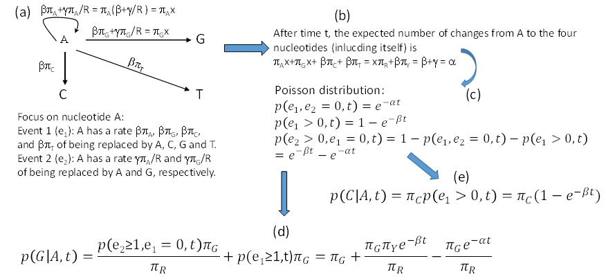 Figure 4: Derivation of transition probabilities based on the F84 model. πA, πG,πC, πT and πR, πY are equilibrium frequencies of A, C, G, T, purine (A + G) and pyrimidine (C + T). Event e1 occurs at a rate of β and leads to the original A being replaced by any of the four nucleotides according to their equilibrium frequencies, and event e2 occurs at a rate of γ and results in the original A being replaced by either A or G according to their frequencies in the purine pool, i.e., πA/πR, and πG/πR. I used x as a shorthand for β+γ/πR. The rate γ does not appear in the final transition probabilities because it has been absorbed into α which equals β+γ shown in (b). P(j|i,t) means the probability of changing from the original nucleotide i to nucleotide j after time t, and is synonymous to pij(t) or simply pij in this paper. View Figure 4
Note that whenever event e1 happens, the original A is replace by A, C, G and T with probabilities πA, πG, πC and πT, no matter how many e2 events has occur before or after the occurrence of e1. This is similar to the scenario involving the K80 model, except that the K80 model assumes equal nucleotide frequencies. It might help to think of a long sequence with L sites being A at time 0. If these L sites each have experienced at least one e2 event, then these sites will either be A or G with probabilities πA and πG, respectively, and we expect to have πAL sites being A and πGL sites being G. In contrast, if each of these L sites has experienced at least one e1 event, then the site will be replaced by A, C, G, or T with probabilities πA, πG, πC and πT, and we expect to observe A, C, G and T in πAL, πGL, πCL, and πTL sites, respectively. Any number of e2 events occurring before or after the e1 event does not change this expectation. This means that e1 erases e2, but not vice versa. The occurrence of an e2 event is informative only when no e1 event has happened.
After time t, the total flow of the original A to the four nucleotides (including itself, Figure 4a and Figure 4b) is
So the probability that no substitution has happened during time t (Figure 4c), according to Poisson distribution, is
The rate of A changing to A, G, C, and T through e1 is βπA + βπG + βπC + βπT = β, so the probability that at least one e1 has occurred during time t is
The probability that e2 has happened but e1 has not is then
The reason for the condition that “e1 has not occurred” is because e1 event can erase e2 event. With these, it is easy to derive transition probability from A to G (Figure 4d) as the summation of 1) A fraction of πG of p(e1 > 0,t), which is the probability of e1 event that results in the original A being replaced by A, C, G, and T with probabilities πA, πG, πC and πT, and 2) A fraction of πG/πR of p(e2 > 0,e1 = 0,t), which is the probability that e2 events not erased by e1. That is,
From now on, p(j|i,t) will be written simply as pij, so p(G|A,t) is pAG. With the same reasoning, we can derive transition probabilities for other A↔G and C↔T substitutions. Note that the two rate parameters in the F84 model (β and γ) have been re-parameterized into α (= β + γ) and β in Eq. (31). The transition probability from the original A to C (a transversion, Figure 4e) is simply
For other transversions, e.g., pAT, one just need to replace πC by πT. The complete transition probability matrix for the F84 model is
Where
As a quick check of the transition probabilities, we first note that when t = 0 (or when α = 0 and β = 0), then the diagonal elements are 1 and all off-diagonal elements are 0, which is what we expected. Second, when t = ∞ with α > 0 and β > 0, then the transition probabilities will approach the equilibrium frequencies, which is also what we expected.
To obtain the distance for the F84 model (DF84), recall that a distance is defined as μt where μ is the average substitution rate, i.e., substitution rates in Eq. (26) weighted by the equilibrium frequencies:
Now we need to obtain βt and γt in order to calculate DF84. We can obtain αt and βt, and then obtain γt = αt - βt, remembering that α = β + γ (Figure 4b and Eq. (27)]. The method we will use is the same as that for the K80 model, i.e., we obtain the expected transitions and transversions, designated E(S) and E(V), respectively, from transition probabilities and equate them to the observed S and V to solve for αt and βt. With the property of time reversibility (e.g., πA•pAG = πG•pGA), we have
Equating E(S) and E(V) to the observed S and V, and solving these two equations with the two unknowns (αt and βt), we have
Substitute βt and γt (= αt - βt) into Eq. (35) and, after some algebraic manipulation, we have a more useful form of DF84:
Where
To illustrate the calculation of DF84, we may use the two aligned sequences in Figure 2 which gives us πA = 6/48, πC = 12/48, πG = 10/48, πT = 20/48, S = 4/24, V = 2/24, αt = 0.5778363341, βt = 0.2076393648, γt = αt - βt = 0.3701969693, and DF84 = 0.3198867427. The variance of the DF84 can be obtained by either the delta method or the method using Fisher information matrix.
A substitution model similar to the F84 model is the HKY85 model, with its rate matrix specified as:
Where (β+γ) is often written as α and the diagonal elements are constrained by each row summing up to 0. The HKY85 model and the F84 model differ only in the specification of rates involving transitions. qAG and qCT are πG(β+γ) and πT(β+γ) in the HKY85 model specified in Eq. (41), in contrast to πG(β+γ/πR) and πT(β+γ/πY), respectively, in the F84 model specified in Eq. (26). By comparing these rates, it becomes obvious that the F84 model would be equivalent to the HKY85 model if πR = πY.
We can obtain the transition probabilities for the HKY85 model in the same way as that for the F84 model. In short, we again start with a nucleotide A and envision two events e1 and e2. Event e1 occurs with rate β, and results in the original A replaced by any of the four nucleotides with probabilities equal to their respective equilibrium frequencies. Event e2 occurs with a rate γ and results in the original A being replaced by either A or G with the probabilities equal to their respective equilibrium frequencies. Fictionalized in this way, the expected number of substitutions after time t is β(πA+πG+πC+πT) + γ(πA+πG) = β+γR. According to the Poisson distribution, the probability that no substitution has happened during time t is
The probability that at least one e1 occurred after time t is
The probability that e2 has occurred but e1 has not is
The transition probability p(G|A,t), abbreviated as pAG, is
In the same way, we can derive other transition probabilities which are shown below:
Where
As a quick check of the transition probabilities, we first note that when t = 0 (or when α = 0 and β = 0), then the diagonal elements are 1 and all off-diagonal elements are 0, which is what we expected. Second, when t approaches infinity with β > 0 and γ > 0, then the transition probabilities will approach the equilibrium frequencies, which is also what we expected.
We cannot derive the distance for the HKY85 model by following the same approach as that for the F84 model. Hasegawa, et al. [4] has tried this approach but were not successful because there is no explicit solution for βt and γt. However, if we treat the A↔G transition and C↔T transition separate, then we can solve for βt and γt [10]. In other words, we obtain one set of βt and γt from observed A↔G transitions and transversions, and another set of βt and γt from observed C↔T transitions and transversions. βt in the two sets are the same as that in Eq. (38), but γt is different between the two sets of estimates. We can then take a weighted average of γt. Admittedly, this does sound mathematically clumsy and explains why HKY85, while commonly used in phylogenetic analysis involving a likelihood framework or Bayesian inference, is almost never used in distance-based phylogenetics.
Here is the somewhat circuitous protocol to get βt and γt from HKY85. The expected numbers of A↔G and C↔T transitions, designated SR and SY, respectively, and transversions are
Setting E(SR) and E(V) to their the observed SR and V, and solve for βt and γt, we have
Where βt is the same as that in Eq. (38), and γRt in Eq. (49) is γt estimated from observed SR and V.
Now we obtain another set of solutions for βt and γt by setting E(SY) and E(V) to their observed SY and V, and solve for βt and γt, we have the same βt but a different γt:
A weighted average of γt could be
The distance for the HKY model
To compute DHY85 using the two aligned sequences in Figure 2, we have πA = 6/48, πC = 12/48, πG = 10/48, πT = 20/48, SY = 4/24, SR = 0, V = 2/24, βt = 0.2076393648, γRt = -0.2223239164, γYt = 1.047432870, weighted γt = 0.624180608, DHKY85 = 0.308904. I intentionally choose the aligned sequences in Figure 2 with SR = 0 just to see if DHKY85 would behave strangely. It did not. For comparison, the same two sequences yield DF84 = 0.319887.
In general, DHKY85 is slightly smaller than DF84. I used the eight vertebrate COI sequences in the FASTA file VertCOI.fas that comes with DAMBE [11] to compute both DHKY85 and DF84 (Figure 5). The difference is minor, although DHKY85 is consistently but slightly smaller than DF84.
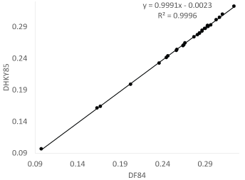 Figure 5: Evolutionary distances from the HKY85 and F84 models are nearly identical. View Figure 5
The HKY85 model itself may not carry much biological significance given the existence of the F84 model. However, the twists involved in computing the evolutionary distance, i.e., the separate estimation of γA↔G and γC↔T, lead very naturally to a very useful TN93 model that we will cover next.
We have come far, so far that we need hardly any extra effort to derive transition probabilities for the TN93 model. There are two equivalent specifications of the rate matrix for the TN93 model. The first is
Where the diagonal elements are constrained by each row summing up to 0. The second specification simply replaces (β + γR/πR) by α1 and (β + γY/πY) by α2. We see that TN93 is reduced to F84 if γR = γY, and to HKY85 if γR / πR = γY / πY.
The similarity between TN93 and F84 allows us to re-use Figure 4 for deriving transition probabilities for TN93. We only need to add a subscript R to γ and α in Figure 4 so that we have γR and αR as rates for purine, keeping everything else the same, and we instantly obtain the transition probabilities for transitional substitutions between purines and for transversional substitutions as shown in Figure 4. To get transition probabilities between pyrimidines, we can just replace the original nucleotide A in Figure 4 by nucleotide C or T and rename γ and α in Figure 4 to γY and αY. Note that our αR = β+γR, and αY = β+γY.
The transition probability matrix for the TN93 model is
Where x1 and x3 are the same as those in Eq. (34), but x2 has α replaced by αR and x4 has α replaced by αY, i.e.,
To obtain the distance for the TN93 model (DTN93), recall that a distance is defined as μt where μ is the average substitution rate, i.e., substitution rates in Eq. (53) weighted by the equilibrium frequencies, so:
Now we need to obtain αRt, &αYt, and βt. The method we will use is the same as that for the K80 and F84 models, i.e., we obtain the expected numbers of A↔G transitions, C↔T transitions, and transversions, designated E(SR), E(SY) and E(V), respectively, from transition probabilities, and equate them to the observed SR, SY and V to solve for αRt, &αYt, and βt:
The resulting αRt, &αYt, and βt are
If one wishes to express DTN93 in SR, SY and V, then one may just substitute γRt, γYt, and βt into Eq. (56), which yields:
Where
To illustrate the application of DTN93 with the two aligned sequences in Figure 2, we have πA = 6/48, πC = 12/48, πG = 10/48, πT = 20/48, SY = 4/24, SR = 0, V = 2/24, αRt = 0.13353, &αYt = 0.90593, βt = 0.20764, γRt = αRt – βt = -0.07411, γYt = αRt – βt = 0.69829, DTN93 = 0.35299. The variance of the DTN93 can be obtained by either the delta method or the method using Fisher information matrix. Note that SR = 0 means no information for estimating αRt properly.
I should mention that all distance formulations in this paper are known as Independently Estimated (IE) distances because they use information from only two aligned sequences and are independent of other pairs of sequences. Practical molecular phylogenetic analysis typically would use Simultaneously Estimated (SE) distances [12,13] which use information from all pairs of sequences. SE distances are implemented in MEGA [14] and DAMBE [11,15]. The PhyPA [16] function in DAMBE, which performs phylogenetic reconstruction base on pairwise alignment when reliable multiple sequence alignment is difficult to obtain for highly diverged sequences, uses SE distances only.
In short, the approach of deriving transition probabilities by probability reasoning can go a long way if one can do good bookkeeping. In particularly, the probability reasoning approach is very useful for conceptual understanding. However, the approach becomes increasing difficult with more complicated substitution models. Two alternative approaches, one involving solving differential equations and the other involving matrix exponential and logarithms, are often used in practical computation with the GTR model for nucleotide sequences and amino acid-based substitution models. They will be numerically illustrated elsewhere.
This study is funded by the Discovery Grant from Natural Science and Engineering Research Council of Canada (RGPIN/261252-2013). I thank C. Vlasschaert and S. Aris-Brosou for feedback.