Reproducibility of results in simulation studies plays a key role in statistical science. Although P-value occupies a prominent place for determining statistical significance in replicate studies, there is always possibility of extra variability across samples leading to irreproducible results. Recently, Halsey, et al. [1] raised issues regarding the reproducibility in the P-value. In this paper, we propose a theoretical basis to identify and adjust for extra variability in simulation studies. Our simulation results show gain (increase in power and reduction in significance level). Although the gain is observed for simulation settings with small sample sizes and less variability with but it is bigger in simulations large samples sizes and high variability. We also discuss the limitations of this 'out of box' solution to increase reproducibility.
Variability reduction, Replication, Monte carlo experiments
Reproducibility of scientific discovery is an important issue in science, medicine, engineering and other fields, which can provide essential validation [2-6]. Despite the importance of reproducibility, there exists the lack of reproducibility for many scientific findings [7-10]. Failure to reproduce results has been a major concern from journal editorial boards [11-14]. Risks with a multiplicity and misinterpretation of the P-values are widespread [15-17]. Extra variability in the P-value may lead to irreproducible results [1]. Thus, the lack of reproducibility presents a fundamental problem in statistical inference. Although inference based on the P-value continues to occupy a prominent place in research, any reports or interpretations may be misleading if scientific findings fails to be reproduced.
Recently, a discussion in the AMSTAT News Publication (AMSTAT News, 2016 Issue 3) issued a statement on the P-value and statistical significance to draw vigorous attention to changing research practices that have contributed to a reproducibility crisis in science. "Widespread use of 'statistical significance' (generally interpreted as 'p < 0.05') as a license for making a claim of a scientific finding (or implied truth) leads to considerable distortion of the scientific process…".
To address this matter, we propose an approach for reduction of extra variability in Monte Carlo experiments. Although our approach presents potentials for Monte Carlo studies, but it can, in principle, be applicable to other replicated (bootstrap) studies. The paper is organized as follows. In Section 2, we describe the issues related to reproducibility in simulation studies. A theoretical approach to reduce variability is introduced in Section 3. In Section 4, we present some results which make a comparison among our approach and the t-tests that are directly applied to the original data. Some concluding remarks are presented in Section 5.
Statistical measures such as P-value, point estimate and confidence interval in replicate studies are not sometimes reliable. The reliability depends on the amount of variability between replicates. To understand the issue, we summarize the results displayed in (Figure 1) from Halsey, et al. [1] in (Table 1). In this simulation study, underlying true means significantly differs. However, in 4 simulations the P-values vary from highly significant to highly not-significant. Furthermore, the P-value reproducibility is affected by the potential outliers and small sample sizes in normally distributed population A (n1) and population B (n2) with (n1 = n2 = 10).
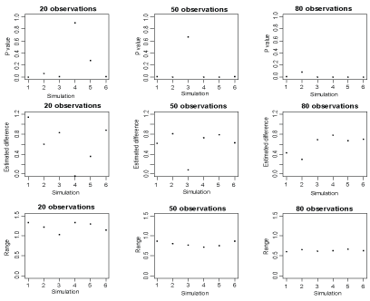 Figure 1: The scatter plot of the P-values, estimated differences in means and ranges of confidence intervals against replicates. View Figure 1
Table 1: Summary of simulation characteristics in Halsey, et al. [1] with η1 = 10 and η2 = 10. View Table 1
To draw statistical inference, we construct hypotheses. Usually the null hypothesis (H0) states that the means in two populations A and B are the same, whereas the alternative hypothesis (H1) states that the means in two populations A and B are different. Using the sample data, we validate these claims. To test these hypotheses, we construct the critical region (range of the mean) and calculate the probability of the critical region under two hypotheses. The significance level, (commonly represented by α), is the probability of the critical region when the null hypothesis is true. The power, (commonly represented by 1-β), is the probability of the critical region when the alternative hypothesis is true.
We expand this example further to study the effect of reproducibility. First, we examine reliability of sample values between replicates. The populations A and B have a common variance of 1 but with different means of 0.5 and 0.0, respectively. From each of the populations A and B, we randomly draw 6 sets of samples of sizes 20, 50 and 80, respectively. Note in this setting (n1 = 20, n2 = 20; n1 = 50, n2 = 50; or n1 = 80, n2 = 80), the power within these settings is 33.8%, 69.7% or 88.2%, respectively, at the significant level alpha = 0.05 for comparing means using a two-sample two-sided t-test.
Figure 2 reports the sample values against 6 replicates for each of the sample sizes from each of the populations. As shown in Figure 2, the sample values markedly vary across replicates, especially for small samples. The values of a large sample drawn from a population might tend to represent that population because the sample is less subject to random variation, while the values of a small sample drawn from a population might not tend to represent that population because in this case, the sample is subject to a random variation. However, whether the sample size is small or large, there exists the variability, with possibility of extra variability, of sample values.
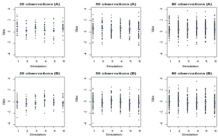 Figure 2: The scatter plot of sample values against replicates, where blue colors represent sample mean. View Figure 2
Next, we examine the variability in P-value, estimated difference and range of confidence interval. Figure 1 reports these statistical measures against replicates with each of the sample sizes. Although the P-values tend to be reliable as the corresponding sample sizes increase, there still exists variability. Similarly, the estimated differences in means vary considerably across replicates even for large samples. The ranges of confidence intervals vary across replicates for small samples as well. These replicate variabilities result variability in the P-values; this issue is discussed at length in the recently published paper in Nature Methods [1].
Further, we examine the effect of sample size on the variability of statistical measures. From each of the populations A and B, we generate 1000 samples of sizes 20, 50 and 80. Figure 3 reports the distributions of the P-values for a two-sided test of the null hypothesis (no difference in means) and the distributions of the point estimates of mean difference along with 95% confidence intervals. We calculate an empirical power, which is defined as the percentage of the replicates where the difference between population means, is declared as a significant effect if the P-value is less than 0.05. The empirical power corresponding to three sample sizes are 34.2%, 68.0% and 88.9%, and are in agreement with the theoretical power. From Figures 1 and Figure 3 we further see that the simulated results tend to be more reliable as the sample sizes increase.
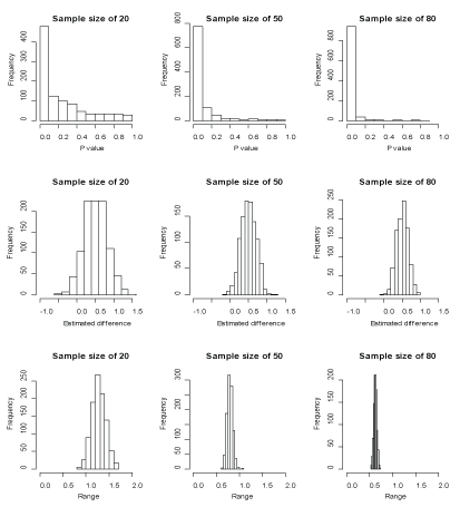 Figure 3: Frequencies of the P-values, estimated differences and ranges for the sample sizes of 20, 50 and 80. View Figure 3
In Figure 1 of Halsey, et al. [1] shows contradicting P-values for smaller sample sizes (n1 = 10 and n2 = 10). Therefore, there is a need for robust replications irrespective of the sample sizes. In the following section, we develop a systematic approach to reduce the variability in replications.
In replicate studies some of the replication may be over dispersed and discarding those should lead to better inference. We develop a systematic approach, in two stages, to evaluate quality of simulations before any estimation. The first stage of our approach, we reduce variability. In the second stage, we apply the commonly used statistical methods such as point estimation, confidence interval and testing-hypothesis on the reduced replicates. In the following, we consider two scenarios: one-sample and two-sample inferences.
Let and let and be the sample mean and standard deviation, respectively, i.e., and . Then, we know that and . Therefore,
and,
Above two equations can be re-represented as
and
where and . Here represents a chi-square distribution with degrees of freedom. Note that and . The expressions in Equation (1) provide a tool to measure the quality of replicated samples.
Now, we define settings and quantitative measures in replicated studies which are generated using parametric bootstrap samples [18]. Let be observation from the population in the bootstrap sample, and be the sample mean and standard deviation of the bootstrap sample, respectively, b = 1, . The two-stage approach to reduce variability is described as follow. If the replicated sample, satisfies at least one condition in equation (2), which is
or
then the sample is called extra-variant and it is removed from further statistical inference.
To estimate the parameters or , we use the grand sample mean, , and the grand sample variance, . Thus, in the first stage, we remove all the possible extra-variation samples and then perform statistical inference. Even though the number of replicate studies (bootstrap size) is predetermined, the resulting bootstrap size will be a random variable. Note that we do not discard individual observations within a sample but discard the entire sample.
and
are estimated and compared in the entire replicates and the reduced replicates.
In the two sample setting let be the , from the population in the bootstrap sample, and be the sample mean and standard deviation from the population in the bootstrap sample, respectively, b = 1, . We compare the quality of each replica,
or
to declare extra-variate pair of samples and to remove from further inference.
As before, we estimate parameters and with and , respectively.
Statistical analyses are performed on the reduced replicates to compare means in one-sample and two-sample settings, which we call it second stage of the entire analysis. This increases the reproducibility in simulation studies. Like in one-sample settings, we estimate and compare
and in the entire replicates and the reduced replicates.
First, the advantage of our two-stage approach can be explicitly visualized in simulation studies. To compare statistical inference for P-value, point estimate or confidence interval using the original replicates and using the reduced replicates, we generated 1000 data sets and each data set includes 20 observations from . We also calculate the P-values for a one-sample t-test where the null hypothesis is that the population mean is zero and the alternative hypothesis is that the population mean is not zero. Figure 4 reports the distributions of the P-values along with the distributions of the point estimates and ranges of 95% confidence intervals for the population means using the original replicates and using the reduced replicates. As shown in this figure, the P-values using the reduced replicates are less variable than those with the original replicates. Also, we gain in power properties using this reduction approach as expected. Furthermore, from an inference point of view, the point estimates and confidence intervals using the reduced replicates are more precise than without reduction. To compare a the P-values for a one-sample t-test using the original data and using the reduced data where the null hypothesis is true, we generate 1000 data sets in which each data set includes 20, 40 and 60 observations from a normal population with mean 0 and variance 1, respectively. Figure 5 reports the P-values using the original data and using the reduced data where the null distribution is true. This figure shows that the P-values using the reduced data are approximately greater than 0.4, which means our approach significantly reduces the type I error (the significant level is 0.05). To compare a the P-values for a one-sample t-test using the original data and using the reduced data where the alternative hypothesis is true, we generate 1000 data sets in which each data set includes 20, 40 and 60 observations from a normal population with mean 0.5 and variance 1, respectively. Figure 6 reports the P-values using the original data and using the reduced data where the alternative hypothesis is true. This figure shows that the P-values for the t-test using the reduced data are approximately smaller than 0.2 for a sample size of 20 and are around 0 for a higher sample size, which means our approach might significantly improve the power, especially for big samples (e.g., sample size = 40 or 60) since power may be calculated as the proportion of p value less than the significance level alpha = 0.05 for data sets where the alternative hypothesis is true. This advantage in power can numerically be confirmed by the results in (Table 2).
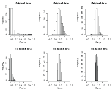 Figure 4: Frequencies of the P-values, sample means and ranges using the original data and using the reduced data. View Figure 4
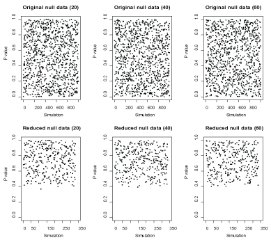 Figure 5: P-values across replicates in the original and reduced null data where the null hypothesis is true. View Figure 5
 Figure 6: P-values across replicates in the original and reduced null data where the alternative hypothesis is true. View Figure 6
Table 2: Comparisons of type I error and power between the one-sample t-test, where Type I error* and Power* represent type I error and power for reduced data, respectively. View Table 2
Next the advantage of our two-stage approach can numerically be shown in simulation studies. To compare a type I error for one-sample t-test using the original data and using the reduced data, we generate 1000 data sets where the null hypothesis is true and in which each data set includes 20, 40 and 60 observations from a normal population with mean 0 and variance 1, respectively. The type I error is calculated as the proportion of P-values less than the significance level alpha = 0.05 for all the 1000 data sets. To compare a power for one-sample t-test using the original data and using the reduced data, we generate 1000 data sets where the alternative hypothesis is true and in which each data set comes from a normal population and the settings of population parameters and sample sizes are given in (Table 2). The results about type I errors and powers are summarized in (Table 2), which shows that our approach reduces drastically type I error because it removes all the abnormal samples prior to perform a t-test and that the powers for the t-test using the reduced data are larger than the ones using the original data. Now we generate 1000 data sets for each of two normal populations A and B with a common standard deviation where the sample sizes from two populations in each data set are the same and the settings of population parameters and sample sizes are given in (Table 3). A similar conclusion is summarized in (Table 3). The powers for the two-sample t-test using the reduced data are larger than the ones using the original data in most cases except when sample size is small (e.g., sample size is 40) or when difference in population means is small (e.g., mean of A is 0.8 and mean of B is 0.6).
Table 3: Comparisons of type I error and power between two-sample t-test. View Table 3
To improve the reproducibility of the results in replicate studies, we propose a two-stage approach to reduce variability. Our simulation studies reveal that the variability of statistical measures such as P value, point estimator and confidence interval has considerably reduced. When compared to one- and two-sample t-test using original data, our approach markedly improve the power and meanwhile reducing potential type I error. Also, the results from statistical inference are interesting. The estimators and confidence intervals of population parameters from one and two populations become more precise after reduction of variability. The reproducibility can be controlled by introducing another parameter, w, in equation (2); i.e.
or
in a one-sample case (a similar representation in two-sample case). In equation (4) different values of will lead to a different degree of reproducibility, which needs to be studied further. As we know the type I and II errors cannot be simultaneously minimized if parameters are fixed, including bootstrap size. However for a fixed type I error, we can select the optimal reproducibility parameter to minize the type II error. Altogether, we discuss practical issues about variability reduction here, it is important to explore the methodology of our approach when studying properties of estimators using bootstrap simulations in a real data.
There are some limitations of the proposed method, an 'out of box' solution for increasing reproducibility. First, the bootstrap size becomes a random variable; how does it compare when using methods based on trimmed data (deleting outliers) for inference is another issue that can be studied further. Also, when the distributional assumptions (normal distribution/Gaussian distribution), are not valid, the method may still work with symmetric and unimodal such as student t-distribution. However, to generalize to a very skewed and/or multimodal distribution requires additional work that one may consider.
Dr. Rai is grateful to generous support from Dr. DM Miller, Director James Graham Brown Cancer Center and Wendell Cherry Chair in Clinical Trial Research.