COVID-19 is the disease caused by a novel coranavirus, which outbreak started in Wuhan community of China during December, 2019. World Health Organisation (WHO) started reporting cases of COVID-19 on 21st January. In this research, we aimed at forecasting new cases of COVID-19 per day, using data collected from 21st January to 10th June, 2020, spanning 142 days, by fitting polynomial models. Different model selection criteria were used to determine the most appropriate model among assumed models. The result of the analysis showed that the cubic model performed better than others. Important plots were displayed to show the fitness of the cubic model to the data. Forecast was made that if there is no new phase of the virus and there are compliances to government policies to prevent the spread of COVID-19 as advised by the Centre of Disease Control (CDC) and WHO, then new cases of COVID-19 per day globally would reduce significantly in coming days. The total confirmed cases would cumulate slowly and reach 11 million before August 2020 as the curve flattens. We recommend that putting on face masks, washing of hands and applying alcohol base sanitisers, cleaning surfaces with disinfectants and keeping physical distance could help to reduce the spread of the virus, thereby flattening the curve.
COVID-19, Cubic regression model, Hierarchical polynomial model, Quadratic regression model, Transmission dynamics
The novel coronavirus, which was isolated on 7th January 2020, is a virus that causes disease called COVID-19, detected in Wuhan City, Hubei Province of China in December, 2019 [1]. A total of 44 cases were reported by World Health Organisation (WHO) China country office from 31st December 2019 to 20th January 2020. WHO received information from National Health Commission China on 11th and 12th January, 2020 that the outbreak is associated with exposures in one seafood market in Wuhan. By 12th January, 2020, China shared the genetic sequence of the novel coronavirus to be used in developing specific diagnostic kits for countries [1].
Thailand reported the first imported case of laboratory confirmed COVID-19 from Wuhan on 13th January, 2020. Japan Ministry of Health, Labour and Welfare (MHLW), on 15th January 2020, reported an imported case of laboratory confirmed COVID-19 from Wuhan. Republic of Korea National Focal Point (NFP) reported the first case of COVID-19 on 20th January 2020. WHO [2] reported on 20th January, 2020 that 282 confirmed cases of COVID-19 from four countries including 278 cases from China, 2 from Thailand, 1 from Japan and 1 from Republic of Korea; all from the same region. Among the 278 cases confirmed in China, 258 cases were reported from Hubei Province (Wuhan), 14 from Guangdong Province, 5 from Beijing Municipality and 1 from Shanghai Municipality; Of the 278 confirmed cases, 51 cases are severely ill, 12 are in critical condition and 6 deaths have been reported from Wuhan [2]. Cases in Thailand, Japan and Republic of Korea are all imported cases from China.
At the moment, most countries of the world are shut-down because of this noisome pestilence called novel coranvirus (COVID-19) because of the rate at which it spreads. The chance of surviving if infected with the virus is high, if the immune system is not compromised. Data since 21st January, 2020 have been officially reported for new and total cases. The spread started from China to border countries, to other continents, and now it has spread all over the continents and the regions of the world, making many big and small countries to shut-down their economies. The virus that was reported officially on 21st January, 2020 with a total reported cases of 282 cases only in Wuhan, has now hit a figure of 7,444,391 cases as at 10th June, 2020, just 142 days after, recording deaths of 416,979, is now in all the continents of the world and in more than 216 countries and territories [3].
United States of America (USA) reported her first case on the 23rd January, 2020, while Australia recorded her first case on the 25th January, 2020. At this point, Italy has not reported any case of COVID-19. The first local transmission was in Vietnam on the 24th January, 2020. The first death outside China was recorded in Philippines on 13th February, 2020. The second death outside China was reported in Japan on 14th February, 2020. Egypt reported its first confirmed case of COVID-19 on the 15th February, 2020. This was the second country in the WHO EMRO region to confirm a case, and the first reported case from the African continent. Lebanon and Israel recorded their first cases on 22nd February, 2020. France recorded the first death in Europe on 22nd February, 2020. The first recorded case in Italy was on 12th February, 2020 and the first death was on 23rd February, 2020 (2 deaths recorded). Algeria is the first Member State of the AFRO Region to report a case of COVID-19 on 26th February, 2020. On 3rd March, 2020, Saudi Arabia recorded her first case [2].
On 26th February, 2020, there were more new cases reported outside of China than in China for the first time, since the onset of COVID-19. On the 28th February, 2020, Nigeria reported the first case of COVID-19 in West African Sub-region, and WHO increased the assessment of the risk of spread and risk of impact of COVID-19 from high to very high at the global level [2].
Rabajante [4] developed mathematical models of COVID-19 dynamics and concluded that the exposure time is a significant factor in spreading the disease with a basic reproduction number of 2, 14-day incubation period, and concluded that if an infected person stay more than 9 hours in the event could infect other people. Jia, et al. [5] adopted three kinds of mathematical models, namely Logistic model, Bertalanffy model and Gompertz model and adjourned logistic model the best among the three models studied and used it to predict the number of individuals expected to be infected in Wuhan, non-Hubei province and in the entire China. Li, et al. [6] established dynamic models of the six chambers, and established the time series models based on different mathematical formulas according to the variation law of the original data and produced results based on time series analysis and kinetic model analysis and used it to predict future spread of the virus.
Sanglier [7] developed models based on multi dimensional adjustment by means of polynomial equations assuming a linear dependence of the function with respect to each of the variables on which it depends in order to assess, in one way or another, the development of epidemics such as that of coronavirus (COVID-19). Hu [8], worked on Artificial Intelligence (AI) forecasting of COVID-19 in China. Chen and Yu [9] studied a second derivative model to characterize the coronavirus epidemic in China with cumulatively diagnosed cases during the first 2 months. Malato [10] predicted COVID-19 infection in Italy using mathematical models and compared logistic and exponential models. Within this few months of outbreak, many authors have worked and published articles on modelling the spread of COVID-19. Among these authors are [11-33].
There are many and different predictive models in statistics. Famoye and Lee [34] opined that some of these models are very useful in predictive analysis, such as, linear models, generalized linear models, mixed models, spline regression, polynomial models, shrinkage regression models, penalized smoothing regression models, regression tree models, unreal network models, random forest models, bagging and boosting modeling techniques, support vector machine methods, and others [35,36]. Most of these predictive models are regression models or time series models or time series regression models.
Disease diffusion is defined as the cumulatively increasing degree of spread of a particular disease among humans or animals from a region of outbreak to other regions, until the disease has spread across all regions (operational definition). If a state of a country is studied, then the regions can be local governments; if a country is studied, then the regions can be states or provinces; if a continent is studied, then the regions can be countries; and if it is a global case, the regions can be continents or countries. In this case of COVID-19, it is a global case, so the regions are the continents, subdivided into countries. All the continents have been affected by COVID-19 as at this period of this research and almost all the countries of the world have been affected. The rate of disease diffusion is the speed at which it spread to all the regions under study at a given time interval from the region of outbreak (operational definition). New cases of the COVID-19 will increase to a maximum point, after which it begins to decrease to zero.
A study area is partitioned into regions, of which the location of the disease outbreak is defined as a region as well. Every region are equal in terms of nomenclature, not in terms of size, strength or economy. These definitions are proposed for this work. Jia, et al. [5] discussed that infectious disease transmission is a complicated diffusion process. So, models developed for studying transmission process of infectious diseases theoretically can be termed as diffusion models. Thus, future development trend of infectious diseases can be accurately predicted. In order to reduce the spread of infectious diseases, the prediction of infectious disease using predictive models is now trending in literature [33]. Kumar [37] described basic model in innovation diffusion as a logistic law of growth that grows exponentially until an upper limit inherent in the system is approached, at which point the growth rate slows and eventually saturates, characterizing S-shaped curve and has broad range of applications.
Faraz, et al. [38] applied analytical solution of linear, quadratic and cubic Model PTT Fluid. Erat [39] applied linear, quadratic and cubic regression models to predict body weight from different body measurements in domestic cats. Trebuna, et al. [40] applied polynomial regression models to prediction of residual stresses of a transversal beam. Ajao, et al. [41] applied polynomial regression model of making cost prediction in mixed cost analysis. Ostertagova [42] applied polynomial regression in modelling the relationship between strains and drilling depth. Gendy, et al. [43] applied polynomial regression model to stabilized turbulent confined jet diffusion flames using bluff body burners.
Most of the authors have not considered modelling the global spread of the novel coronavirus using polynomial regression models, and the authors that have applied polynomial regression models have not applied it to modelling COVID-19 transmission rate at global level.
Thus, in this research, we fitted hierarchical polynomial regression models on daily cases of COVID-19 globally and forecast new cases in coming days. The world is assumed to be a global village, that can be influenced by a single government. This is evident in the spread of the virus from China to other part of the world, as if there were no physical boundaries. Also, the whole world is fast complying to CDC and WHO policies as if we were under one world government. The data collected is a time series data because it is collected on regular time interval (in days) but it is fitted by a regression model. So, it can be regarded as a time series regression model. Polynomial models are types of regression models, in which the simple linear regression is a special case. A polynomial regression model is hierarchical if all the terms of the independent variable raised to a power are all present in the model. In this case, the observation, yt is dependent on t and higher powers of t. It is a diffusion model because the rate of spread is time dependent. As time t increases, the spread measured in number of persons per time unit (say yt) also increases until it has saturated to maximum, and any further increase in t will result to decrease in yt. Since, it is not a theoretical model, in real life, there could be increase and decrease between small change in t, but in the long run, it shows a pattern that can be modelled by the so called diffusion model.
The rest of the paper is written as follows. The methodology is given in section 2, where the assumed models were discussed as well as some important properties of diffusion models, such as the survival function, hazard function, reversed hazard function and cumulative hazard function; the results were displayed in section 3, where the COVID-19 data was analyzed, the best model was selected and a forecast was made. Section 4 is the discussion of the results while in section 5, we gave some concluding remarks and made some recommendations based on the result of the model and WHO recommendations.
Coronaviruses were first identified in the mid-1960s and were known to infect humans and a variety of animals, including birds and mammals. Since 2002, two coronaviruses infecting animals have evolved and caused outbreaks in humans viz-a-viz SARS-CoV (2002, Betacoronavirus, subgenus Sarbecovirus), and MERS-CoV (2012, Betacoronavirus, subgenus Merbecovirus) [44]. In 2002-2003, SARS-CoV affected 8,096 people, causing severe pulmonary infections and 774 deaths (case fatality ratio: 10%) [44,45]. Coronavirus is likely to originate from bats, then spread to Himalayan palm civets, Chinese ferret badgers and raccoon dogs sold for food at the wet markets of Guangdong, China. MERS-CoV was identified in 2012 in Saudi Arabia and since then the majority of human cases have been reported from the Arabian Peninsula. In healthcare, human-to-human-transmission has been the main route of diffusion of the virus. Although, dromedary camels are also intermedtiary hosts of the virus. The case fatality ratio of MERS-CoV infections is estimated at 35% [46,47].
The virus that causes COVID-19 was first isolated in December 2019 from three patients with pneumonia, connected to the cluster of acute respiratory illness cases from Wuhan, China. Genetic analysis shows that the novel coronavirus is related to SARS-CoV and genetically clusters within the genus Betacoronavirus, forming a distinct clade in lineage B of the subgenus Sarbecovirus together with two bat-derived SARS-like strains [48,49]. The origin of the virus is not clear yet. Similar to SARS-CoV, a recent study confirmed that Angiotensin Converting Enzyme 2 (ACE 2), a membrane exopeptidase, is the receptor used by 2019-nCoV for entry into the human cells [50].
COVID-19 is an infectious disease caused by a novel coronavirus. The virus is believed to be zoonotic in origin, from bats to intermediate host to humans [51]. The virus was initially isolated in bronchoalveolar lavage fluid samples [49,50]. RNA of the virus was detected in blood samples in six out of 41 cases in a study of the clinical features of the infection [52]. So far, it remains unknown if the virus is excreted in faeces or urine. The schema of the flow of COVID-19 virus from animal to human is depicted in Figure 1.
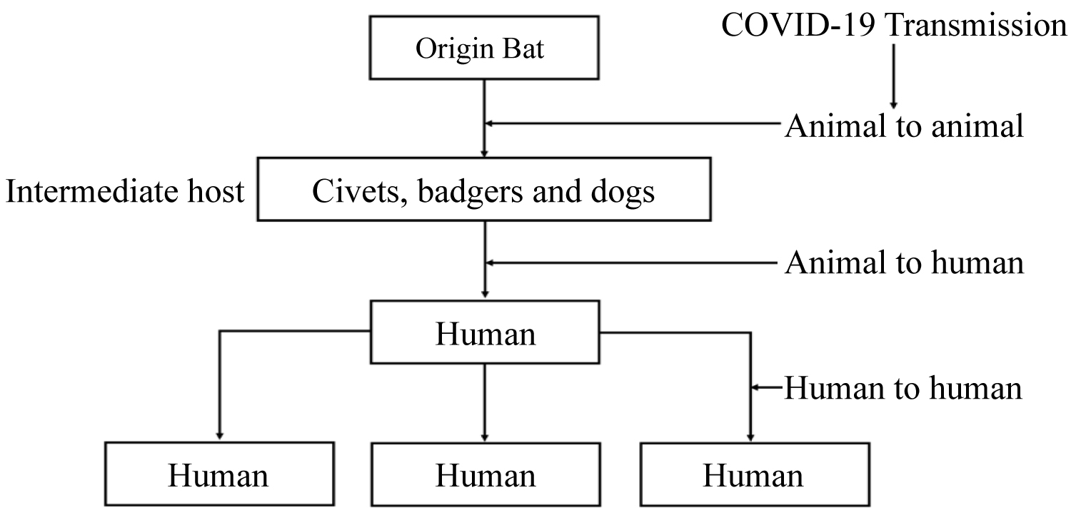 Figure 1: History of coronavirus transmission from bat to man. Source: Authors.
View Figure 1
Figure 1: History of coronavirus transmission from bat to man. Source: Authors.
View Figure 1
Figure 1 shows that an infected human has the possibility of transmitting it to 3 other humans, and each of the 3 newly infected humans can infect other 3 humans with the virus, and this trend can continue if no drastic action is taken to stop the spread. Liu, et al. [53] estimated mean of basic reproduction number (R0) for COVID-19 as around 3.28, with a median of 2.79. The basic reproduction number, R0 represents, on the average, the number of individuals an infected person can transmit the virus to. It represents the average number of new infections generated by an infectious person in a totally naïve population [53].
Also, the following authors got different R0, [54] R0 is 6.49, [53] R0 are 2.90 and 2.92, [55] is 3.11, [56] is 2.55, [57] is 1.95, [58] is 4.08, [59] are 2.24 and 3.58, [60] is 2.5, [61] is 6.47 and [62] is 2.2. The mean of these different R0 is 3.42 and the median is 2.91. Thus, it can be said that the basic reproduction number, R0 for COVID-19 is approximately 3 globally.
The spread is believed to be geographically associated, but with uncertainty. Human-to-human transmission of COVID-19 has been established, such as through respiratory droplets, and there is also a suspicion of asymptomatic infection. The symptoms of COVID-19 include mild to moderate respiratory illness. Infected individuals recover without requiring special treatment. Older people who immune system have been compromised with underlying medical problems like cardiovascular disease, diabetes, chronic respiratory disease, and cancer are more vulnerable to develop serious illness and eventually die. The mode of transmission of the COVID-19 virus is primarily through droplets of saliva or discharge from the nose when an infected person coughs or sneezes. At the moment, there are no specific vaccines or treatments for COVID-19. Nevertheless, the virus has been isolated in the lab and many advances has been made in evaluating potential treatments [4]. The isolated novel coronavirus is depicted in Figure 2.
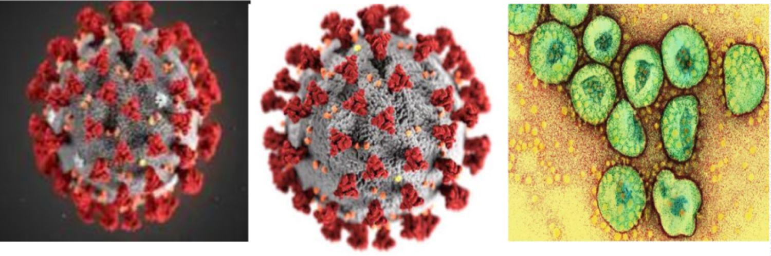 Figure 2: Isolated coronavirus. Source: Nature Magazine 2020.
View Figure 2
Figure 2: Isolated coronavirus. Source: Nature Magazine 2020.
View Figure 2
The virus has been exported from China to other parts of the world through travel-related activities [3]. On 30th January 2020, the WHO declared COVID-19 outbreak as a 'Public Health Emergency of International Concern', specifically to enhance the level of preparedness of countries that need additional support [2]. To prevent the global spread of the virus, many countries have imposed travel restrictions to and from China. Initially, many countries issued temporary travel ban starting on 2nd February 2020 to flights coming from and going to China, including Hong Kong and Macau. Today, many countries of the world have completely extended the band to other countries to stop imported cases.
WHO and CDC have gained experience from previous outbreaks due to other coronaviruses (Middle-East Respiratory Syndrome (MERS) and Severe Acute Respiratory Syndrome (SARS), that human-to-human transmission occurred through droplets, contact and fomites, suggesting that the transmission mode of the COVID-19 can be similar [2]. The suggested basic principles to reduce the general risk of transmission of COVID-19 following previous outbreak of coronavirus include the following:
• Social distance (physical distance of atleast 1 metre apart).
• Frequent hand-washing, especially after direct contact with infected people or their environment or surfaces.
• Keep away from farm or wild animals, except you are protected.
• Cough etiquette should be practised by people with symptoms of acute respiratory infection (cover coughs with disposable tissues or clothe, and wash hands).
• Emergency unit in hospitals should enhance standard infection prevention and control practices.
• Stay at home policy.
WHO and CDC did not give any recommendation to travellers but it is expected that are encouraged to seek medical attention and share their travel history with the centre of disease control (CDC) in their country of residence.
The flowchart in Figure 3 shows that bats transferred the virus to dogs, civets, etc, (not scientifically proved), humans became infected by coming in contact with the infected animals (secondary host). The infected humans infect other humans in the same region (local transmission). The infected humans travelled to other regions where the borders are not closed (these infected humans are counted as imported cases in the new region) and the infected imports infect humans in the new region who come in contact with them. The new infected humans can infect other humans in their region that have contact with them (local transmission). The stay at home policy is as a result of border not closed. If individuals comply to the stay at home policy, then the spread stops, but if otherwise the spread continues. The infected humans can either die or recover depending on their immune system and method of medication.
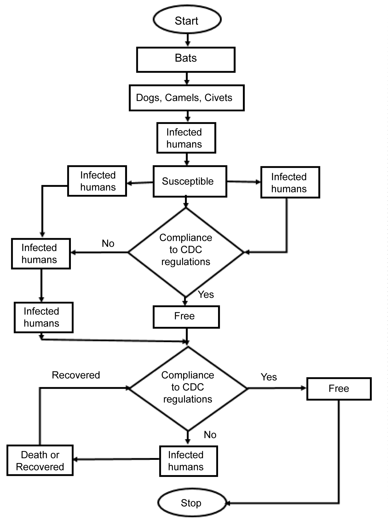 Figure 3: Flowchart showing COVID-19 transmission dynamics.
View Figure 3
Figure 3: Flowchart showing COVID-19 transmission dynamics.
View Figure 3
The novel coronavirus has been grown in cell culture by Peter Doherty Institute for Infection and Immunity in Melbourne, Australia. They are the first outside China to achieve this feat. The novel coronavirus was isolated from the first person diagnosed with the infection in Australia, on 25th January [63].
The team will share the virus with other research laboratories around the globe as recommended by the WHO to help the development of more accurate diagnostic tests and vaccines [1,63]. With the virus already isolated, it would be much easier to find exact cure for it. Many progresses had been made in mathematical science, which would aid the medical science in producing vaccines for the virus [1].
Onofri [64] in his work title ”some useful equations for nonlinear regression in R” mentioned that curves can be easily classified by their shapes, which could be used in selecting the most appropriate model for the process under study. These models are polynomials, such as linear, quadratic, cubic, quartic models; Concave/Convex curves (with no point of inflection), such as exponential, asymptotic, negative exponential, power curve, logarithmic, rectangular hyperbola; sygmoidal curves, such as logistic, Gompertz, log-logistic, Weibull; and curves with a maximum, such as Brain-Cousens models. Note that under sygmoidal curves other models, especially the convoluted models can be classified in this type such as Beta-Weibull [65], Weibull-Logistic [66], Normal-Weibull and Weibull-Uniform [67], Weibull-Normal and Logistic-Normal [68,69], Weibull-Cauchy [70], Weibull-Exponential and Logistic-Exponential [71], Odd Lomax-Exponential [72] and reduced beta skewed laplace [73]. Unfortunately, most of these distributions predictive models have not been developed.
Nevertheless, after looking carefully at the plot of the data seeing the curve, three models were selected from the polynomial models and they are hierarchical polynomial regression models. The three hierarchical polynomial regression models assumed to fit the COVID-19 new cases data are the linear (a line), the quadratic (a parabola) and the cubic models. These three models are hierarchical polynomial models of order one, two and three respectively. They are also diffusion regression models. The three models are linear in parameters but are not linear in variables.
Polynomial regression is a special case of multiple regression, with only one independent variable t [42], with the dependent variable yt linearly depending on the powers of the single independent variable (t, t2, ..., tk). One-variable polynomial regression model with kth order can be expressed as
where yt is the measured or observed variable at time t and k is the order of the polynomial, the βs are the unknown parameters to be estimated. The et is the error term, which is also time dependent and follows the probability distribution of yt. Note that t is a time sequence (t = 1,2,3,...,n). If k = 1, then equation (1) becomes
Equation (2) is a simple linear model (polynomial of order 1). The method of Least square (LS) is the best linear unbiased estimator (BLUE) and it would be used to estimate the model parameters. Equation (2) is the population model, the realization from (2) can be estimated by
Equation (3) has linear effect parameter β1 and the constant parameter β0.
Definition 1: A hierarchical quadratic model is a polynomial of degree 2 with all the terms present. If k = 2, and all the terms are present, then equation (1) becomes
Equation (4) is a quadratic equation or polynomial of order 2. The method of Least square (LS) is also used to estimate the model parameters, because the model is linear in parameters. Equation (5) is the population model of (4), the realization from (4) can be estimated by
Equation (5) has the linear effect parameter β1 and quadratic effect parameter β2 respectively as well as the constant parameter β0.
Definition 2: A point of inflection is a point where a function changes concavity.
Note that:
1. A line has no concavity.
2. A parabola has no inflection point.
Definition 3: A hierarchical cubic model is a polynomial of degree 3 with all the terms present and is defined by
the fitted model is given by
Note that a cubic function has exactly one point of inflection.
The parameter β0 = E(yt) when t = 0 and it can be included in the model provided t passes through the origin, that is, t = 0 exist. If t = 0 does not exist, then β0 has no meaning.
A basic assumption in linear regression analysis is that rank of variance covariance matrix is full column rank. In polynomial regression models, as the order increases, the variance covariance matrix becomes illconditioned. As a result, its inverse may not be accurate as G-inverse might be used and parameters will be estimated with considerable error. If values of t lie in a narrow range then the degree of ill-conditioning increases and multicollinearity in the columns of T matrix enters. A model is said to be hierarchical if it contains the terms t, t2, t3, etc. Hierarchical models are invariant under linear transformation. This is why it is expected that all polynomial models have this property. This requirement is more attractive from mathematics point of view. One of the assumptions in usual multiple linear regression analysis is that all the independent variables are linearly independent [74]. In polynomial regression model, this assumption is not satisfied. Even if the ill-conditioning is removed by centering, there may exist still high levels of multicollinearity. Such difficulty is overcome by orthogonal polynomials.
Consider the polynomial model of order k in one variable as
This model can as well be written in matrix form as
y = TB + e (9)
where T is a matrix of the independent variable and the columns of T will not be orthogonal. If we add another terms then the matrix has to be recalculated and consequently, the lower order parameters will also change.
In particular, consider this diffusion hierarchical cubic model given by
It is a diffusion model because yt increases with time and would reduce when maximum yt is reached. A diffusion model has the ability to spread at a higher rate from the point of discharge until a maximum point is reached. At this point, the spread has been saturated and the rate of spread decreases. It is a hierarchical model because all the terms of t are included, meaning βk ≠ 0 for k = 1,2,3. It is a cubic model because the highest power of t is 3, that is, it is a polynomial of order 3.
The model expressed in equation (10) can be fitted as
where and are the least square estimates of β0, β1, β2 and β3 respectively.
These parameters can be estimated as follows.
Note that equation (10) is dependent on time, such that t1 = 1, t2 = 2, t3 = 3. For easy derivation of the least square parameters, without loss of generality, equation (10) can be written as
The function is the kth order orthogonal polynomial defined as
and T matrix from equation (10) is given by
Since this T-matrix has orthogonal columns, so the variance covariance, matrix becomes
The least square estimator of B in matrix form is given by
where is a column vector of s, such that,
A special case is if j = 0, we have
where are the least square estimates of respectively.
The variance of is given by
where unknown σ2 can be estimated from the analysis of variance (ANOVA) summary table (Table 1).
Table 1: Analysis of Variance (ANOVA) table. View Table 1
where is the residual sum of squares, and
where is the regression sum of squares, and does not depend on other parameters in the model.
The total reported cases of COVID-19 from inception to time t is the cumulative of the newly reported cases to time t and it is denoted by F(t). It is a non-decreasing function, irrespective of f(t), since f(t) ≥ 0 ∀ t. The survival function is the number of survivor from COVID-19, that is, the susceptible class, not yet infected by COVID-19, but are in treat of the disease and it is given by
S(t) = N - F(t) (13)
where N is the total population under study. Here, N = 7.8 billion persons, the population of the world as at June, 2020. Also, h(t) is called the pressure function or the hazard function. The growth is proportional to the susceptible population (potential COVID-19 infected). The hazard function of a diffusion model describes the factor affecting the growth in the spread of the COVID-19 disease. The hazard or pressure function h(t) characterizes the structure of the diffusion model of COVID-19 and it is defined by:
The number of outbreak of COVID-19 in a neighbourhood of t, conditional on the outcome (yt) being no more than t is called the reverse hazard function and it is given by
The cumulative hazard function is the derivative of h(t) with respect to t and it is given by
In this section, data were collected from WHO (2020) and Worldometers (2020) on COVID-19 daily reported cases from 21 January 2020 to 10 June 2020, spanning 142 days as shown in Appendix I. Data on new cases, new deaths and new recovered on daily basis were collected and analyzed. Exploratory Data Analysis (EDA) of the data collected were carried out as preliminary analysis. Predictive models were formulated by choosing the best model from 4 competing models using the following goodness of fit and model selection criteria, coefficient of determination (R2), log-likelihood, Akaike Information Criterion (AIC), Bayesian Information Criterion (BIC), Kolmogorov Smirnov (K-S) statistic and P-value. The 4 competing models are simple linear regression, quadratic regression, cubic regression with a constant term (Cubic 1) and cubic regression without a constant term (Cubic 2).
The exploratory data analysis (EDA) are carried out in this section using descriptive statistics and various charts, including time plots to show some hidden features in the datasets. Table 2 displays part of the data collected on COVID-19.
Table 2: New cases of COVID-19. View Table 2
Figure 4 are plots that show hidden features of the datasets. Figures a, b and c are histograms, e, f and g are boxplots, while h, i and j are density plots of new COVID-19 cases, new COVID-19 induced deaths and new COVID-19 recovered cases respectively. The plots show bimodality of the datasets. This bimodality of the COVID-19 datasets opens new area of research to T-R{Y} and T-X family of probability distributions (Table 3).
Table 3: Descriptive statistics on COVID-19 data. View Table 3
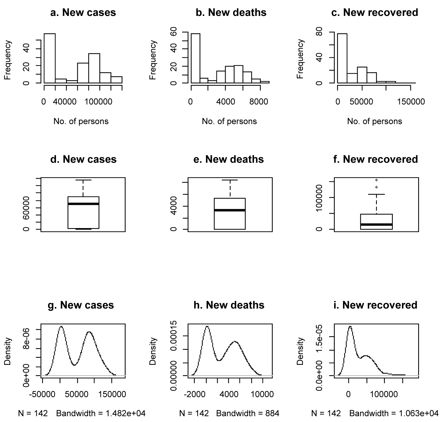 Figure 4: Exploratory data analysis plots.
View Figure 4
Figure 4: Exploratory data analysis plots.
View Figure 4
Five countries each were selected from six regions, Europe, North America, Asia, South America, Africa and Oceania to show each region situation report as shown in Figure 5 and the data are displayed in Appendix II.
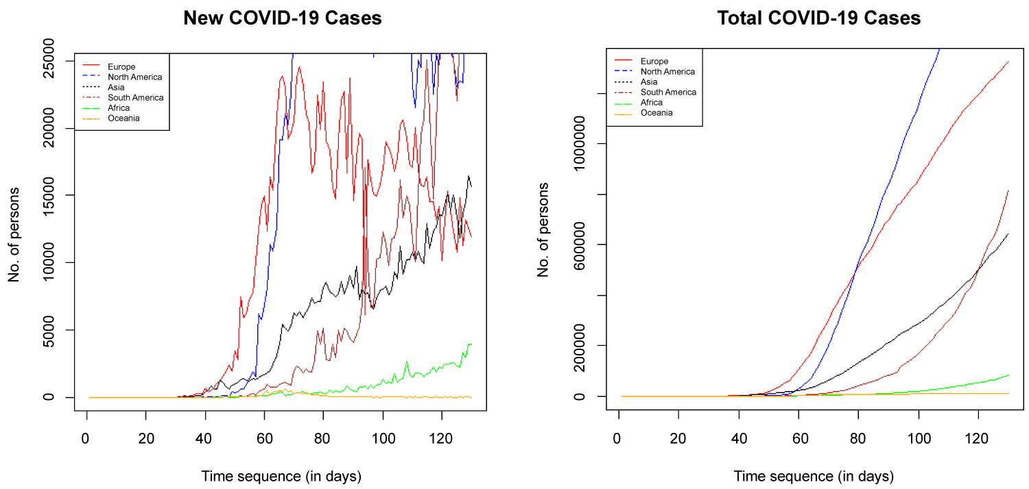 Figure 5: Time plot of new and total COVID-19 cases by region.
View Figure 5
Figure 5: Time plot of new and total COVID-19 cases by region.
View Figure 5
The three competing models are estimated using the least square estimation techniques and the results of the parameters estimated are displayed in Table 4.
Table 4: Least square parameter estimates, F-Test and P-value. View Table 4
Table 5 shows that it is only Cubic 1 that adequately fit the COVID-19 daily cases data. Cubic 2 has the highest coefficient of determination and the lowest AIC, and BIC, making it the best model using these criteria. Cubic 1 on the other hand has the lowest-LogLikelihood and highest KS p-value, making it the best fitted model to the data. Since the model is to be used for predicting and forecasting purposes, Cubic 1 is selected as the most appropriate model for this research. Thus Cubic 1 is used to forecast future occurrence of COVID-19 new cases globally.
Table 5: Measure of goodness of fit and model selection criteria. View Table 5
Let be the estimated COVID-19 daily case at time (t,), the model for COVID-19 daily cases fitted is therefore given by
Equation (17) shows that if t = 0, f(0) = 3287.5, the number of new COVID-19 cases globally will be 3,288 at a steady state of the infection (when time effect is not felt). At the moment, we are in a transient state of the virus (time effect is felt). Equation (17) also shows that number of reported new COVID-19 cases will decrease by 758 daily provided other factors affecting COVID-19 are kept constant (Figure 6).
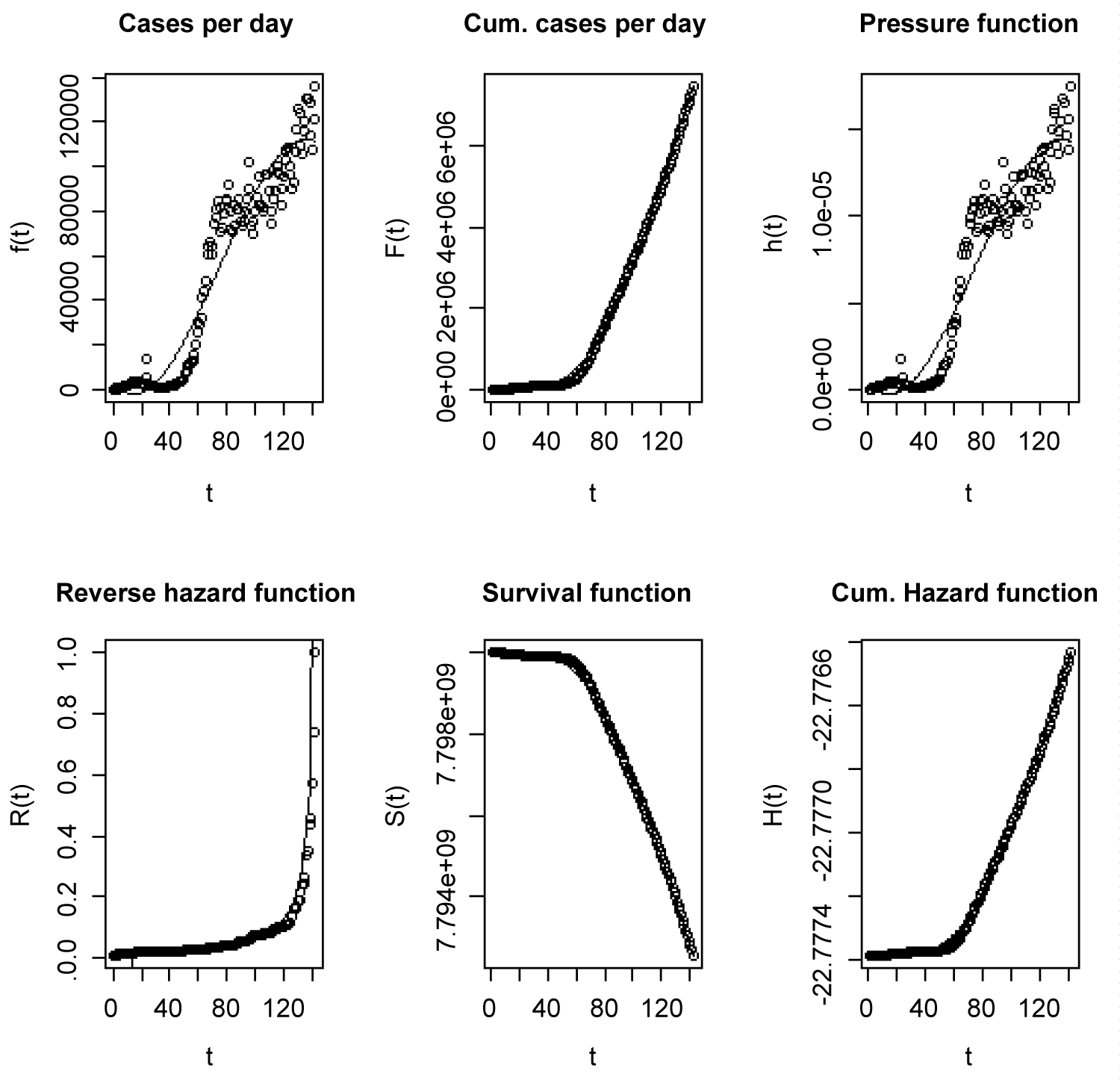 Figure 6: Plots of properties such as pressure and related functions.
View Figure 6
Figure 6: Plots of properties such as pressure and related functions.
View Figure 6
Let T be a random variable representing the time duration of the spread of COVID-19 around the world (measured in days), then the survival function S(t) is the number of people that would remain without the virus for at least t days. The pressure or hazard function h(t) is the number of individuals that would be infected with the virus in the next instant, conditional on having remained without the virus until time t. The reverse hazard function R(t), gives the number of individuals that would be infected with the virus during the interval (t-dt, t), conditional on being infected for no longer than t days. The cumulative hazard function shows negative values because of the negative of the log of values greater than zero are used. The cases per days are new cases reported on daily basis, while the cumulated cases per day are all reported cases from the day of first reported case to time t.
The model fitted in equation (17) is the most appropriate model selected for prediction and forecasting of COVID-19 rate of transmission globally. The fitted model is used to forecast for the coming months as shown in Figure 7.
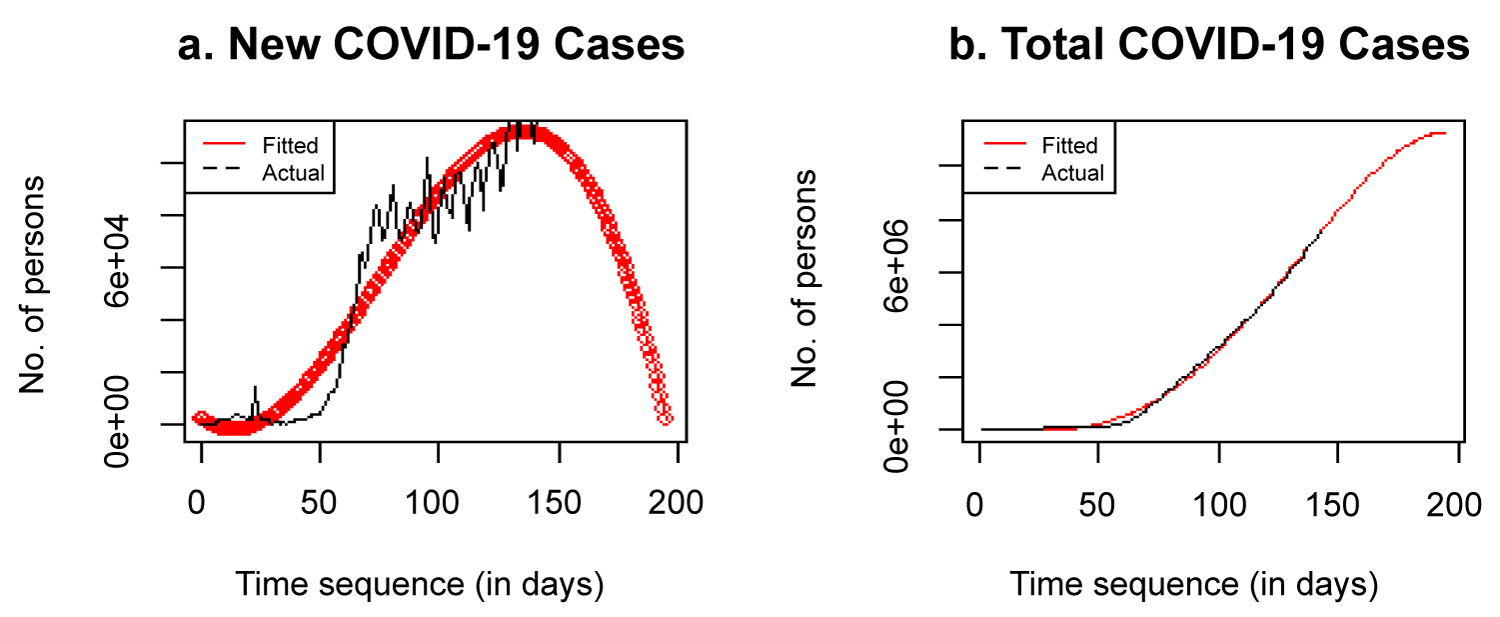 Figure 7: a) Forecast of new cases; b) Forecast of total cases.
View Figure 7
Figure 7: a) Forecast of new cases; b) Forecast of total cases.
View Figure 7
Table 2 shows that new cases of COVID-19 reported as at 21 January 2020 was just 60 per day, while by 10 June 2020, it has risen to 135,578 reported cases per day. Only 3 COVID-19 induced deaths and no recovered cases were recorded on 21 January 2020 but by 10 June 2020, COVID-19 induced deaths per day has risen to 5,163 and recovered cases per day has risen to 131,298.
Table 3 shows that the average number of reported new COVID-19 cases per day is 52,424 for the period under review with coefficient of variation of 84.62% and a very high standard deviation of 44,359.23. The average number of reported COVID-19 induced deaths per day is 2,937 for the period under review with coefficient of variation of 90.13%. The average number of reported COVID-19 recovered cases per day is 27,866 for the period under review with ccoefficient of variation of 114.24%. The three variables newly infected cases, new deaths and new recovered cases are positively skewed.
Figure 8 shows time plots of the three variables and the fourth plot shows the combined plots of the log of the three variables (new cases, deaths and recovered). The new cases and recovered plots are trending up, while that of death is trending down. Both deaths and recovered depend on infected individuals. If there are no COVID-19 infected individuals, there would not be COVID-19 induced deaths and there would not be COVID-19 recovered individuals. So, the trend on new cases need to be studied and forecast.
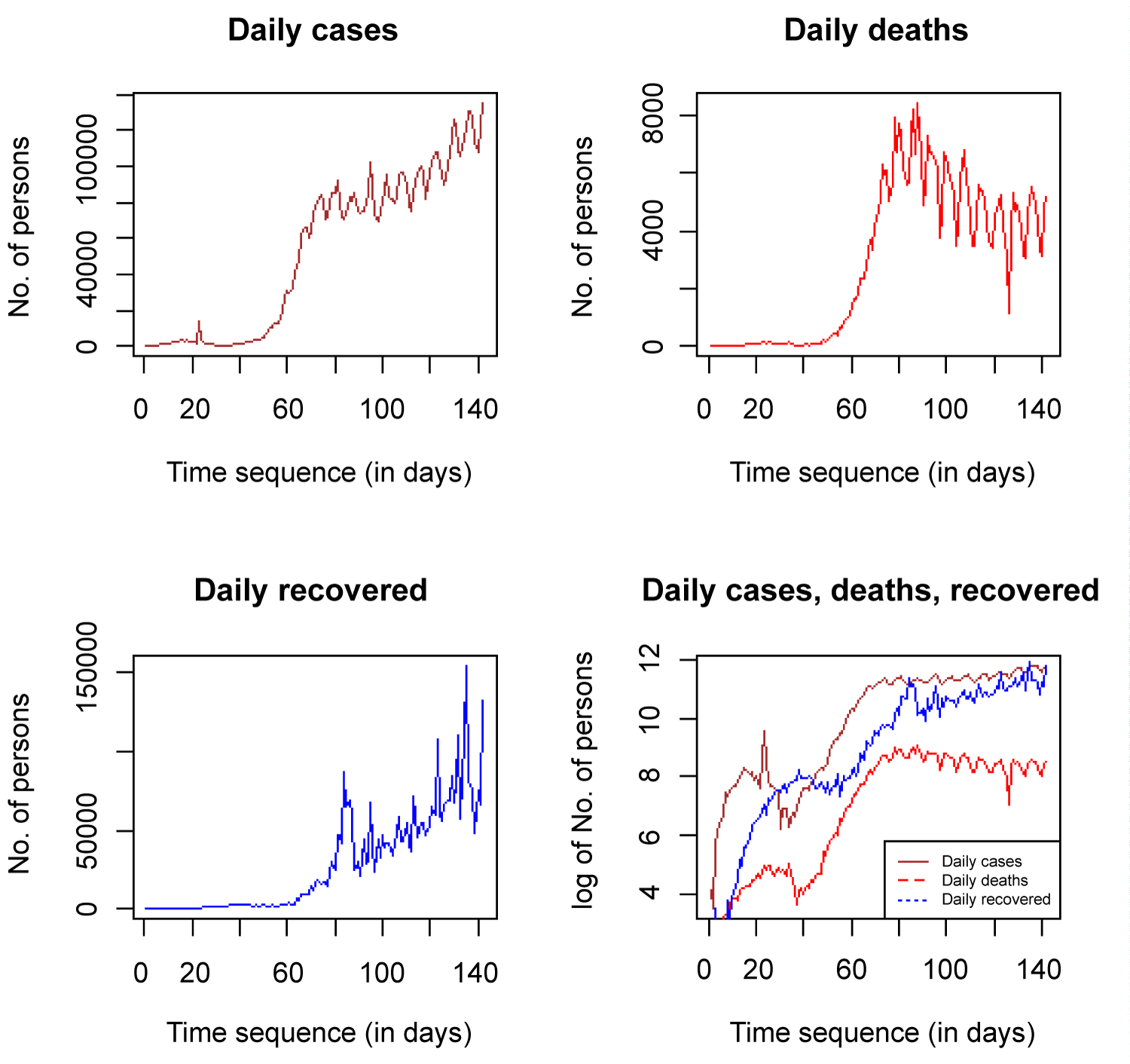 Figure 8: Time plot of new cases, new deaths, new recovered and combined.
View Figure 8
Figure 8: Time plot of new cases, new deaths, new recovered and combined.
View Figure 8
Figure 9 shows time plots of the total COVID 19 cases globally for the three variables and the fourth plot shows the combined plots of the log of the total cases (infected, deaths and recovered). All the plots did not plateau at the ceiling, rather, they are moving towards the ceiling as t → ∞. The total number of deaths and total recovered cases must be less than the total infected individuals as depicted by the combined plot. The active cases individuals are the ones left after the total deaths and total recovered have been subtracted from the total infected individuals.
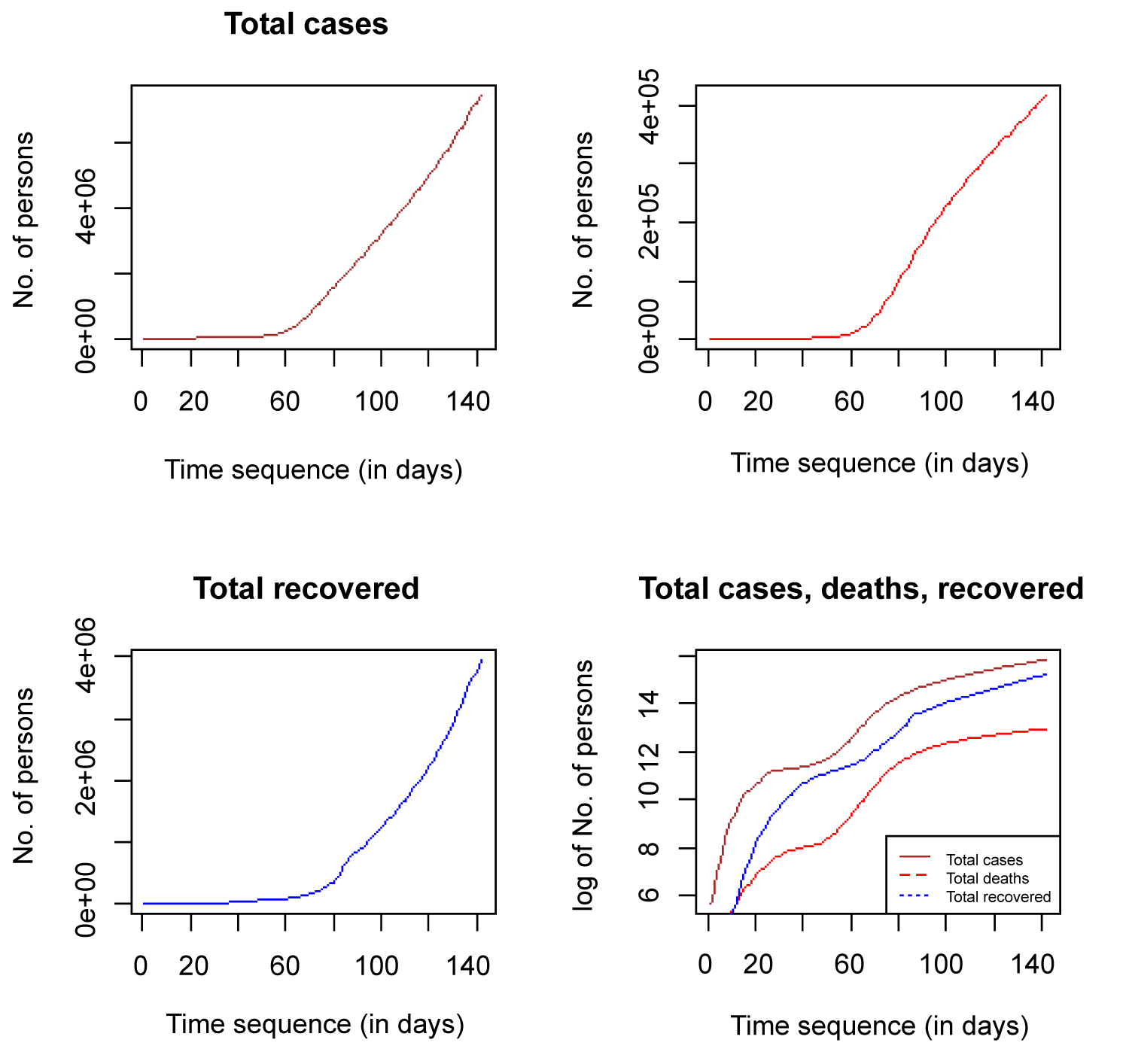 Figure 9: Time plot of total cases, total deaths, total recovered and combined.
View Figure 9
Figure 9: Time plot of total cases, total deaths, total recovered and combined.
View Figure 9
Figure 10 (a) shows that the probability of death is decreasing while the probability of recovery is increasing. If the probability of recovery is success, p, then the probability of death is failure q, such that p + q = 1, where p = recovered cases/closed cases. Note that closed cases = recovered cases + deaths. For the first 10 days of the report deaths and recovered cases are interchanging but after the first 10 days, as t tends to infinity, the probability of recovery tends to 1 and that of death tends to zero.
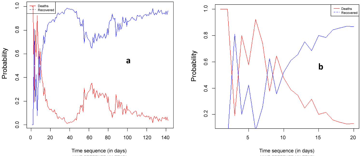 Figure 10: Time plot of probability of death and recovered.
View Figure 10
Figure 10: Time plot of probability of death and recovered.
View Figure 10
Figure 5 is a time plot showing new cases total cases placed side by side. The new COVID-19 cases plot shows that Europe, North America and Oceania have reached their peak as regions and are trending down, flattening the total cases curve. However, Asia, South America and Africa have not reached their peaks as regions.
Table 4 shows that all the 4 models are significant, meaning that the relationship between f(t) and t is significantly different from zero. All the F-test p-values are less than 0.05. Note that The major different between Cubic 1 and Cubic 2 is that Cubic 1 has constant term, while Cubic 2 does not have a constant term, meaning that f(0) = 0. Both Cubic 1 and Cubic 2 are the most significant models among the 4 competing models. They satisfy the non-negative condition of f(t), that is, f(t) ≥ 0. Number of new cases cannot be negative. Number of persons infected with COVID-19 are positive integer values. Based on the fitness of the models to the data using KS statistic and p-value, we selected Cubic 1 as the most appropriate model.
Figure 6 depicts that the graph of the cumulated cases would plateau at the top if the number of new cases becomes zero. As it were, the number of new cases are still going up. The number of new cases, total cases, pressure function, reverse hazard function, survival function and cumulative hazard function are depicted in Figure 6.
All the plots depicted in Figure 11 show that the selected model (Cubic 1) is a good fit for the data. The histogram with the density plot on it, QQ, PP, and TTT plots all showed good fit.
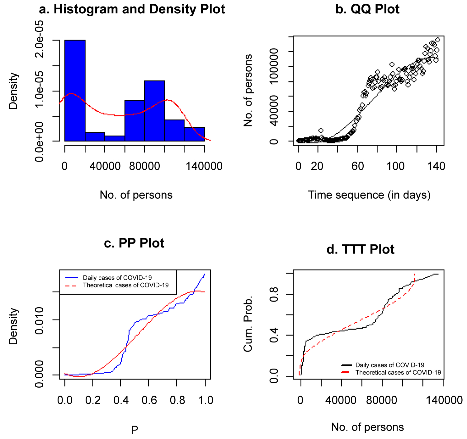 Figure 11: Histogram, QQ, PP and TTT plots of COVID-19 new cases.
View Figure 11
Figure 11: Histogram, QQ, PP and TTT plots of COVID-19 new cases.
View Figure 11
Figure 7 shows that the spread of COVID-19 globally would increase to a maximum and beginning to decrease significant to as low as 2,000 new cases in some months to come, if no new phase of the virus emerges as a result of easing lockdown globally. This will slow down total cases, which is expected to reach 11 million before August. At this point, the curve is flattened as new cases reduce, the total cases increase at a slower rate, making the curve to look like the cumulative frequency curve, because it is a non-decreasing curve. It is very clear that everything cannot remain the same as many countries of the world will begin to reopen their economy and ready for the post-pandemic era. The stay at home policy was a drastic action taken by many countries of the world to reduce the spread of the virus. The rate of spread is decreasing as compared to its rate earlier this year. If the spread continues at a slower rate, it would take no time to reach the zero point. The result shows that the virus might not be completely wipe out but can be reduced to a very insignificant number, with many people developping natural immunity to it. In Africa, the initial and major cases were imported with little local transmission, but now, all African countries have been infected with the virus through local transmission. If all African countries can comply to CDC and WHO regulations, first many local transmission would be reported, after which African countries would begin to record fewer new cases and eventually zero cases. There are still many research to be done with African data on COVID-19, especially on dynamic mathematical models to control the rate of diffusion of the virus.
There are still many research to be done with African data on COVID-19 and other conutries or regional data, especially on dynamic mathematical models to control the rate of diffusion of the virus. COVID-19 is an infectious disease that can be model by dynamic mathematical models. Giordano, et al. [75] modelled COVID-19 pandemic and implemented population-wide interventions in Italy. Dehning, et al. [76] revealed the effectiveness of interventions on the spread of COVID-19, evident from significant change points.
The spread of noisome COVID-19 across the globe is a thing of conern to WHO and the entire global economy. The way the disease has spread since it was first discovered in Wuhan China to the remaining part of the globe is worth studying. The spread of COVID-19 on a time plot is an upward trend, with some inherent pattern within some days. This spread is time dependent and need a diffusion model to fit its rate of spread or how much it would spread within some specified time periods. Three models were fitted on new cases of COVID-19 collected from 21 January 2020 to 10 June 2020, covering 142 days. The result of the analysis showed that the cubic model with a constant term is selected as the best model to predict the spread of COVID-19 globally. The number of deaths and the number of recovered cases can only be derived from the infected classes. Note that f(t) ≥ 0 and a constant negative term cannot make sense in real world situation. It can be best explained that when t = 0, then f(t) = 0. This is the point before the first reported case.
The model was used to predict the spread of the virus in the coming months and the number of COVID-19 reported new cases will decrease to as low as 2,000 globally in coming days, provided countries of the world comply to WHO and CDC directives. This prediction is very much possible if drastic steps are taken to reduce the spread. It is advisable that there should be mass testing in every susceptible population. So, the only way to stop the trend of spread of COVID-19 is to abide by the WHO recommendations of physical distance and the stay at home policy for all countries with increasing new cases, but countries with decreasing new cases should reopen their economies based on WHO and CDC recommendations. A complete locked down of all the countries of the world would be the best option, until the spread begin to experience a downward trend. My recommendation to stop the spread is that if I stay at my home, you stay at your home, he stays at his home, she stays at her home and they stay at their home, then coronavirus would have no medium for transmission and reported new cases would reduce naturally as t becomes larger. Thus, f(t) would tend to zero as t tends to infinity. We also recommend that putting on face masks, washing of hands and applying alcohol base sanitisers, cleaning surfaces with disinfectants and keeping physical distance of at least 1 metre could help to reduce the spread of the virus, thereby flattening the curve.
We acknowledge all the sources of data, especially the World Heath Organisation (WHO). We are also grateful to Lagos State Polytechnic for giving us the platform to do our research. We also want to acknowledge Department of Mathematics, University of Lagos, Nigeria and Department of Statistics University of Ilorin, Kwara State, Nigeria where Mr. Matthew Ekum and Mr. Adeyinka Ogunsanya are currently running their PhD in Statistics respectively.