Hierarchical Bayes Approach for Analysis of Item-Level Missing Data

Junshan Qiu

doi:10.23937/2469-5831/1510009

International Journal of

Clinical Biostatistics and Biometrics ISSN: 2469-5831

RESEARCH ARTICLE | VOLUME 2, ISSUE 1 | OPEN ACCESS DOI: 10.23937/2469-5831/1510009

Hierarchical Bayes Approach for Analysis of Item-Level Missing Data

Junshan Qiu* and Ram Tiwari

Office of Biostatistics, Center for Drug Evaluation and Research, USA

^*Corresponding author: Junshan Qiu, Office of Biostatistics, Center for Drug Evaluation and Research, 10903 New Hampshire Ave, Silver Spring, MD, USA.

Accepted: June 28, 2016 | Published: June 30, 2016

Citation: Junshan Q, Ram T (2016) Hierarchical Bayes Approach for Analysis of Item-Level Missing Data. Int J Clin Biostat Biom 2:009. doi.org/10.23937/2469-5831/1510009

Copyright: © 2016 Junshan Q, et al. This is an open-access article distributed under the terms of the Creative Commons Attribution License, which permits unrestricted use, distribution, and reproduction in any medium, provided the original author and source are credited.

Abstract

In evaluation of neuropathy, change in neurologic function over time has been assessed using validated scores such as the Neuropathy Impairment Score (NIS), the NIS plus 7 (NIS + 7) and the modified NIS + 7 (mNIS + 7). These scores can be further categorized into sub-scores (i.e., domains). Each domain is composed of multiple questionnaires (i.e., items). Scale scores that sum or average a set of questionnaire items are used to address their substantive questions. Missing data could happen at not only the item level but also at the scale level if a visit is completely missed. In addition, same types of missingness often occur in the patient-reported outcomes. Multiple imputations at both the item and the scale levels have been implemented to generate complete data for making inference. Here, we propose a fully Bayesian approach, hierarchical Bayes, to handle the item-level missing data, and to make inference on each domain and across all the domains. In addition to testing the performance of the proposed approach using simulation studies, the proposed approach is applied to a publically available data.

Keywords

Patient-reported outcomes, Domain, Item-level missing data, MCMC, Residuals

Introduction

Types of missing data

Missing data are primarily due to dropout which can be categorized into different types based on its relation to the response process. For simplicity, it is generally assumed that the relation between a specific type of dropout and the response process can be described using a single (indicator) random variable. In case of distinct types of dropout, it is natural to use the multinomial indicator variables to model the dropout. In addition, monotone missing pattern is a key requirement for most of the methods for handling missing data, especially in the longitudinal data analyses. However, this assumption is not required for the sectional setting where only the observations collected at a single time point are of the primary interest.

Missing data in multi-item questionnaires

Multi-item questionnaires have been widely used to measure either investigator- or patient-reported outcomes (PROs) as the sum or average of a total score. Missing responses to certain items in the questionnaires generally occur due to a variety of reasons, particularly in the PROs. In case of missing responses to some of the questions/items in a multi-item questionnaire, the calculation of the total scores could be completed via simply ignoring the missing values or with imputation of missing values. Regardless of the reasons for the omitted responses, analyzing an incomplete data without addressing the missing items may result in misleading results, depending on the extent of missingness. McKnight and McKnight [1] recommended making diagnosis of missing data to distinguish three situations: ignorable given a few missing items, treatable given a reasonable amount of missing items, and non-treatable given a large swath of missing items. Averaging over the available items is often advised given that the items are all expressed in a common metric, and the scale is uni-dimensional and having acceptable consistency or convergent validity (e.g., Cronbach's alpha is sufficiently high, at or above 0.70) [2]. It is equivalent to put equal weights over the items given the assumptions are valid. However, this method can result in biased results when there are deviations from the aforementioned assumptions (e.g., inflated estimates of inter-item consistency) or when the missing completely at random assumption (MCAR) is not valid [3]. To overcome this problem, using non-missing consistent or convergent items to directly estimate an imputed score has been recommended [2]. A complete-case analysis is another option. Similar to the averaging over available cases, this method can result in not only biased analyses when data are not MCAR but also suboptimal power of the study [4].

Furthermore, a big proportion of missing item scores can lead to missing total scores at scale level. As such, missing data in a multi-item questionnaire needs to be handled at the item level and/or at the scale level. Previous studies have demonstrated that precision will improve when missingness is handled at the item level [5]. There are two main approaches used to handle the missing data at the item level: one is to use a full information maximum likelihood (FIML) approach; and the second method is to include the item-level information as a parcel or complete summary score of the available items in case that the number of included item scores is large [3,6]. The second method models the item information as auxiliary variables [7]. The concept of the second method is inspired by Collins et al. [8], who recommend that researchers should routinely include variables in the missing data model if they have high correlations with the variables containing missingness, whether or not they are part of the cause of missingness. As such, the plausibility of missing at random (MAR) is increased.

Most of the items in the questionnaire consist of a small number of ordered categories and can be treated as ordinal variables. As long as the amount of missing data is not extensive and the marginal distribution is approximately uni-modal and symmetric for each item, we can use a normal model to impute the missing data and make inference using the imputed multi-item data [9].

Handling missing data in Bayesian paradigm

From a Bayesian perspective, missing values are treated as unknown quantities, and hence random variables, for which a joint posterior distribution can be derived; or missing data are treated as latent variables that can be included as part of the complete data. Thus, the distinction between the missing data and unknown model parameters is not obvious. Using the OpenBUGS, the Markov chain Monte Carlo (MCMC) samples from the joint posterior distribution of the model parameters and missing values can be generated. In other words, the missing part of the data can be simulated from its conditional posterior distribution given the observed data, and other model parameters. Under a fully Bayesian paradigm, any inference will be based on the conditional posterior distributions of interested quantities directly, while certain multiple imputation approaches relying on the models for imputation of missing values make inferences based on multiple imputed datasets [10]. As such, a fully Bayesian approach seems more straightforward than a two-stage multiple imputation approach.

The proposed fully Bayesian approach is analogous to the multiple imputation approach based on the method known as fully conditional specification [10] and is presented in the next Section on Bayesian Modeling. The performance of the proposed approach is assessed in Section on Evaluation of Model Performance with respect to residuals; and inferences on quantities of interest such as overall treatment effect, are compared with the corresponding Frequentist inferences. Sensitivity analyses are also conducted to evaluate the robustness of the proposed approach on missing data mechanism. In Sections on Examples and Real Data Analyses, we further demonstrate how to implement the proposed approach.

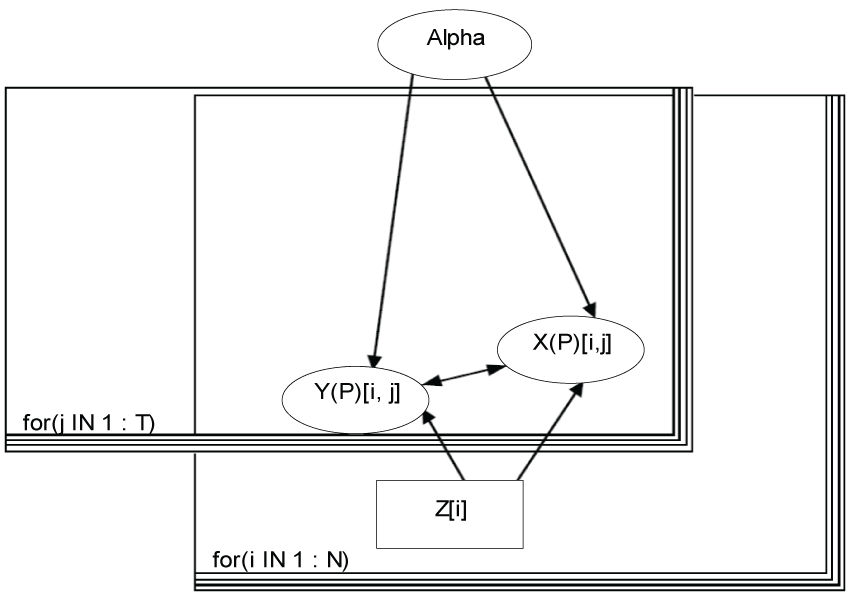Figure 1: Bayesian modeling. View Figure 1

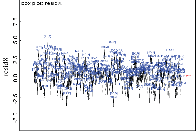Figure 2: Residual plot for domain X under the null. View Figure 2

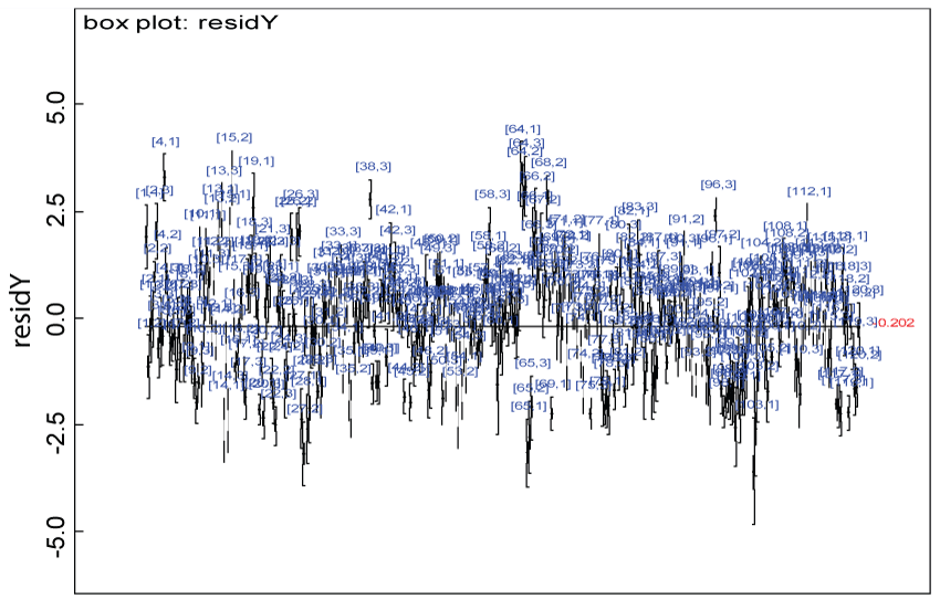Figure 3: Residual plot for domain Y under the null. View Figure 3

Bayesian Modeling

Model structure

To start with a simple example, we assume that there are two domains (X and Y) assessed by the 5-level scores, and three items within each domain (j = 1, T) with T = 3. Each item mean at individual level (Y(X)Pij) can be expressed as a linear function of other items and covariates, Z, such as treatment, age, gender, etc., as in Equations (1.1) and (1.2):

$Y P_{i j} = α_{j 0} + {α^{'}}_{j, [1, T - 1,]}^{} Y {(P)}_{i (- j)} + {α^{'}}_{j, [T, 2 * T - 1]}^{} X {(P)}_{i .} + {α^{'}}^{}_{j, [2 * T, 2 * T + M]} Z_{i} (1 .1)$

$X P_{i j} = α_{j 0} + {α^{'}}_{j, [1, T]}^{} Y {(P)}_{i .} + {α^{'}}_{j, [T + 1, 2 * T - 1]}^{} X {(P)}_{i (- j)} + {α^{'}}^{}_{j, [2 * T, 2 * T + M]} Z_{i} (1 .2)$

Here M is the total number of covariates; Y(P) and X(P) represent the variables that are either observed as Y or X, or derived as YP or XP (e.g., predicted mean via Monte Carlo sampling); and Y(X) means that the data could be from domain Y or X. We assume that Y_ijk or X_ijk are observed for subject i (i = 1,...,N; and N is the total number of subjects enrolled) in treatment group Z_i = k on item j, and that Y_ijk or X_ijk follows a normal distribution with a mean YP_ijk or XP_ijk and a common precision τ, which is specified as a fixed number. That is, $Y {(X)}_{i j} | Z_{i} = k, τ \sim N o r m a l (Y (X) P_{i j k}, τ), k = 1,2 .$

We model the number of missing observations per subject, u[i] using a categorical distribution with a parameter vector calpha. $u [i] \sim d c a t (c a l p h a [Z [i], 1 : b]),$

where b = 3; calpha [Z[i], 1: b] follows a Dirichlet distribution with a parameter vector which has each element of 1.

The model is displayed in figure 1.

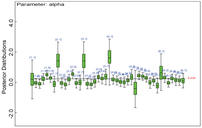Figure 4: Posterior distributions of parameter alpha. View Figure 4

Figure 5: Boxplot of posterior distributions of treatment effects in domain X. View Figure 5

Figure 6: Boxplot of posterior distributions of treatment effects in domain Y. View Figure 6

Prior distributions

To accelerate model convergence, we assume that the elements of the vector, α, are independent and follow a truncated normal distribution with mean 0 and precision 0.001 with range of L to U. That is,

$α_{j j' .} \sim N (0, 0.001) I (L_{α}, U_{α})$

where L_α and U_α refer to the upper and lower limits of the truncation range for parameter $α j j'; j$ refers to the item as the response variable, $j'$ is the explanatory variable, and I(A) refers to the indicator of the set A.

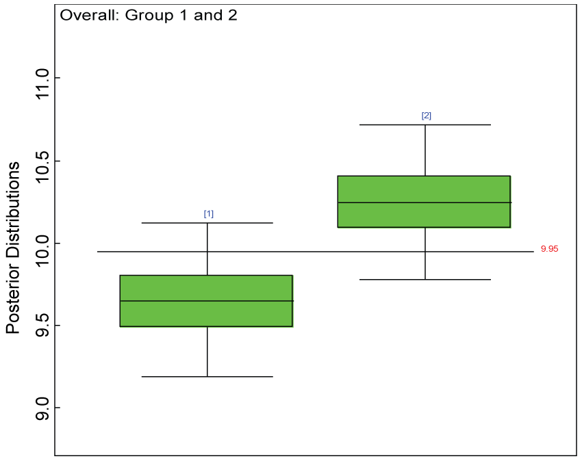Figure 7: Posterior distributions of overall treatment effects. View Figure 7

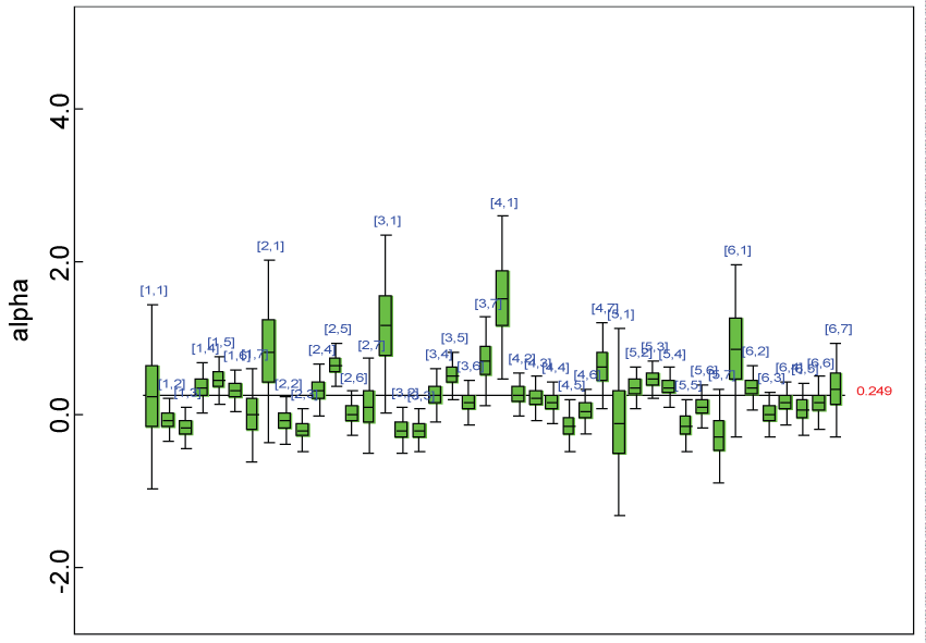Figure 8: Posterior distributions of model parameters. View Figure 8

Mechanism: Relay from completely to partially observed sets

Prior to fitting the model above, the data set was divided into sections by missing patterns as in table 1 with "1" indicating missing and "0" indicating observed.

Table 1: Missing Sections 9 to 16. View Table 1

Table 2 demonstrates how the missing values are predicted. The procedure is summarized step by step as follows.

Table 2: Relay algorithm. View Table 2

1. Start from complete set 1, under Column "Section", namely S1, which includes the subjects who have all the assessments for each item within each domain. The Bayesian model is used to generate the predicted values at item level within each domain for the subjects in S1. There is no specific order required in generating these values. YP^d[Sm, j] or XP^d[Sm, j], within each cell in table 2, symbolizes the predicted values of item j within domain Y or X for subjects in set m, where d is the order number of the prediction for set m.

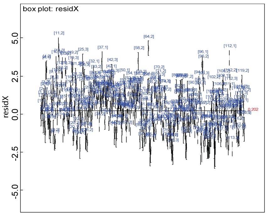Figure 9: Residual plot for domain X under the harmonized alternative. View Figure 9

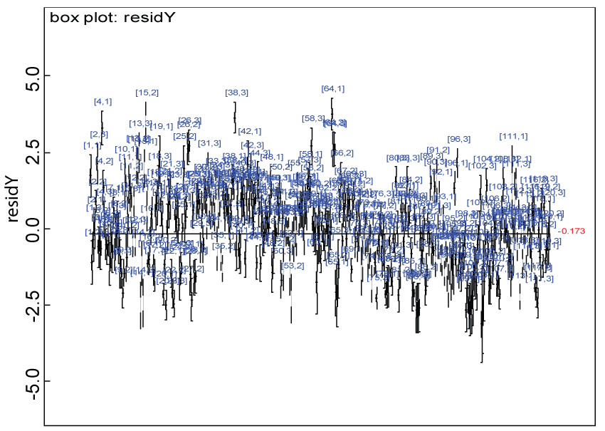Figure 10: Residual plot for domain Y under the harmonized alternative. View Figure 10

2. For set 2, S2, YP¹ [S2, 1] is estimated first using the observed values of other items across the domains Y and X, and the Bayesian model. The YP¹ [S2, 1] serves as imputed values for next estimation which would be based on Y¹ [S2, 1] if observed. The remaining items across the domains will be modeled following the procedure in Step 1. The same procedure is repeated for S3 to S7.

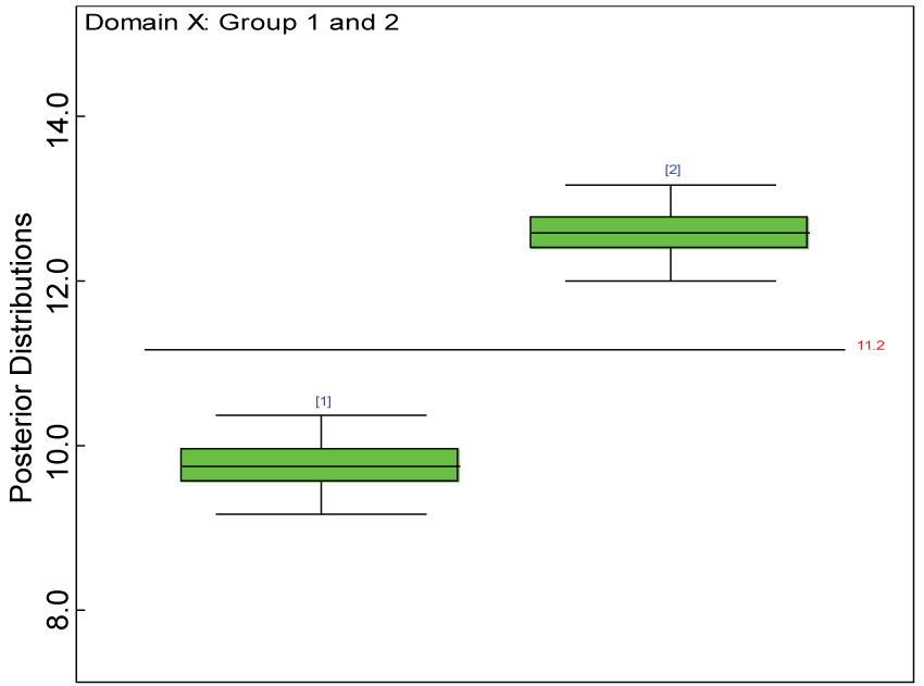Figure 11: Box plot of treatment effect for domain X under the harmonized alternative. View Figure 11

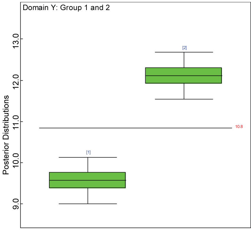Figure 12: Box plot of treatment effect for domain Y under the harmonized alternative. View Figure 12

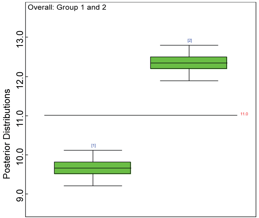Figure 13: Posterior distributions of overall treatment effects. View Figure 13

3. Starting from S8, there are two missing items across the domains. The first step is to borrow the mean of the observed item values for S1 or from all the sections to impute the corresponding item in S8. If the groups are heterogeneous, it is better to borrow within each group. Then the second missing item is predicted with the remaining observed item values and the imputed item value, X¹[S8,1], following the procedure in Step 2. The same procedure is repeated for S9 to S16.

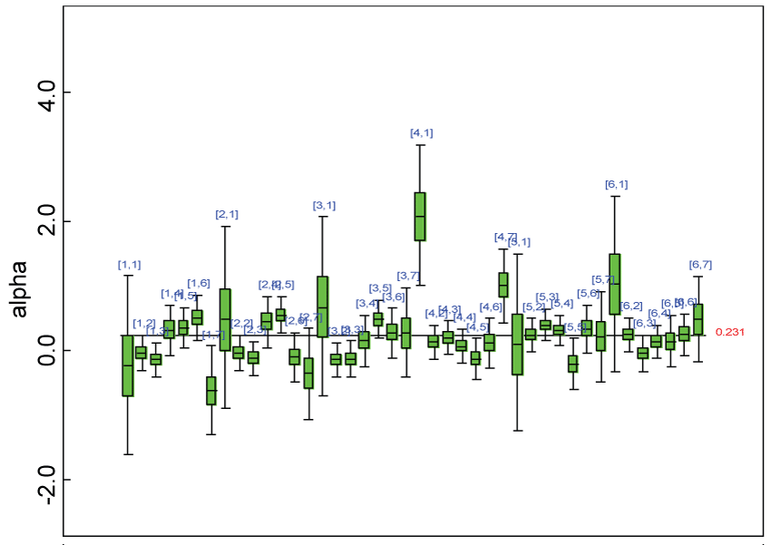Figure 14: Posterior distributions of parameter alpha. View Figure 14

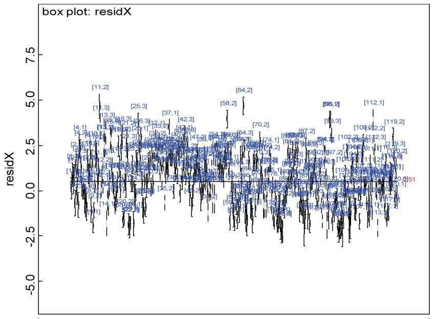Figure 15: Residual plot for domain X under the heterogenic alternative hypothesis. View Figure 15

Note that this procedure can be easily generated to more than 2 domains and more than 3 items per domains.

Figure 16: Residual plot of domain Y under the heterogenic hypothesis. View Figure 16

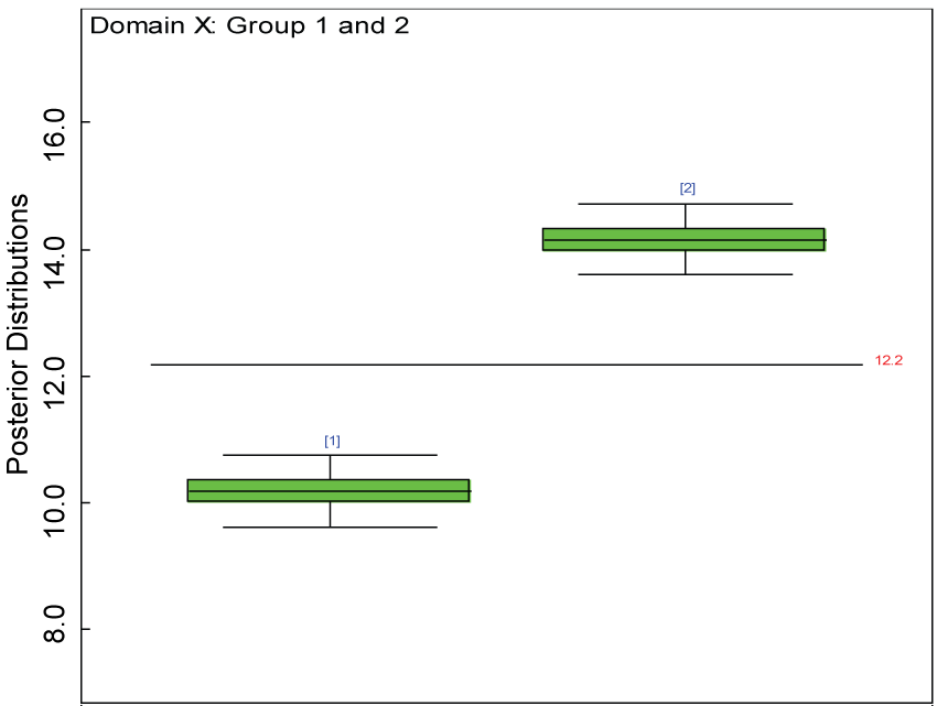Figure 17: Box plot of treatment effect of domain X under the heterogenic hypothesis. View Figure 17

Evaluation of model performance

Before making any inference based on the posterior distributions, convergence must be achieved for the MCMC simulation of each chain for each parameter. In addition, if the MCMC simulation has an adaptive phase, any inference is made using values sampled after the end of the adaptive phase. The Gelman-Rubin statistic (R), as modified by [11] is calculated to assess the convergence by comparing within- and between-chain variability over the second half of each chain. This R statistic will be greater than 1 if the starting values are suitably over-dispersed; it will tend to 1 as convergence is approached. In general practice, if R < 1.05, we might assume convergence has been reached. The MCMC simulation for each model parameter is examined using the R statistic. The convergence of the MCMC simulation for each model parameter of interest is identified for inferences.

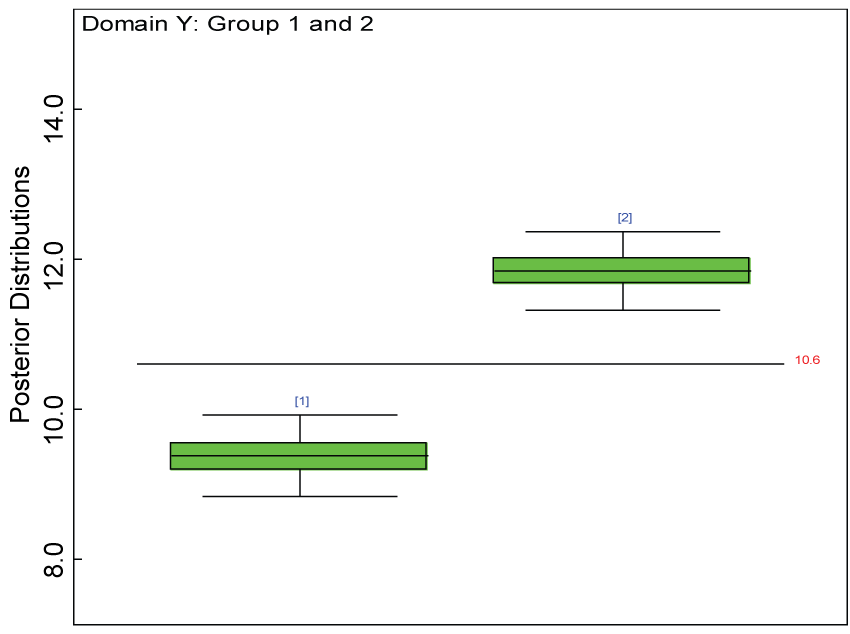Figure 18: Box plot of treatment effect for domain Y under the heterogenic hypothesis. View Figure 18

Figure 19: Posterior distributions of overall treatment effects. View Figure 19

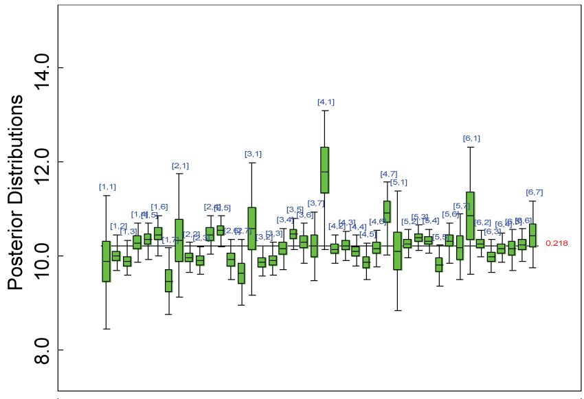Figure 20: Posterior distributions of parameter alpha2. View Figure 20

To assess the performance of the hierarchical Bayesian model, we plotted the residuals, which are defined as the difference between the predicted mean for each subject and each item and the corresponding simulated observations. To evaluate the proposed approach for handling missing data, we check whether the false positive rate for detecting treatment effect under the null hypothesis can be controlled at the desired level; and whether the power for detecting treatment effect at the desired level under the alternative hypothesis can be retained at least. In addition, the Bayesian analyses results are compared with the frequentist counterpart.

Figure 21: Posterior distributions of parameter alpha. View Figure 21

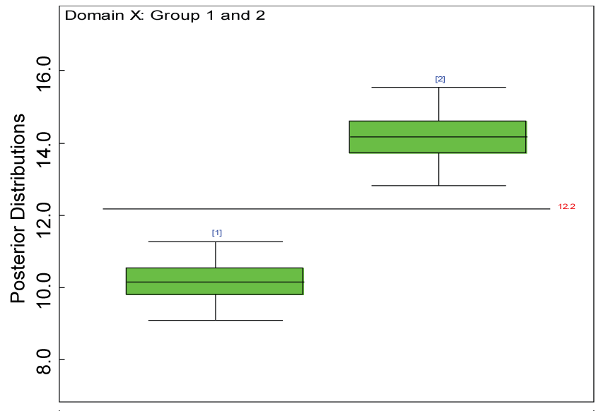Figure 22: Posterior distributions of treatment effects for domain X under MNAR. View Figure 22

Checking residuals

The prediction ability of the hierarchical Bayesian model plays an important role in handling missing data because the predicted mean will be used to impute the missing values. If the residuals are small in magnitude, the imputed values will be close to the true values of the missing observations and will result in inferences with better precision and less bias. We use the following equation to define residuals for Subject i and Item j

$R e s i d Y [i, j] = Y P [i, j] - Y S [i, j]$ where YP[i,j] refers to the predicted mean for Subject i and Item j, and YS[i,j] refers to the simulated observation for Subject i and Item j.

Inference: Detecting treatment effects

Gibbs sampling was used to make inferences because it is hard to find an analytical solution to the hierarchical model with parameters at multiple levels. After checking whether the posterior distributions of model parameters have converged and whether the imputed values are close to the true values of missing observations, we can decide whether this hierarchical Bayes model can be used to make sound inferences. Our primary interest of inference is on detecting treatment effects at each domain and overall levels.

We carried out simulations in two main categories: under the null hypothesis: no treatment effect within each domain and under the alternative hypothesis: significant treatment effect within each domain.

Comparing with the frequentist results

Analysis of Variance (ANOVA) was used to test the treatment effect within each domain at the significance level of 0.05. The analyses results were compared with their counterparts from the Bayesian analysis. Instead of using p-values, the 95% lower and upper bounds of credible intervals for average domain scores were used. If the 95% lower bound of the credible interval for the treated group is greater than the 95% upper bound of the control group, the treatment effect is statistically significant in favor of the treatment.

Figure 23: Posterior distributions of treatment effects for domain Y under MNAR. View Figure 23

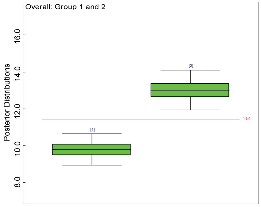Figure 24: Posterior distributions of overall treatment effects under MNAR. View Figure 24

Sensitivity analyses

Given that the full data distribution can be factored into an extrapolation model and an observed data model, one or more parameters indexing extrapolation may not be identified by the observed data [12]. Parameters indexing missing data extrapolation are called sensitivity parameters, in general. This concept is used to assess sensitivity of model-based inferences to either assumptions about missing data mechanisms or informative prior distributions. Under the assumption of MAR, the corresponding constrains require that the conditional distribution for a missing observation $p_{\geq 2} (X_{i j} | X_{i, (- j)}, Y_{i .}) or p_{\geq 2} (Y_{i j} | Y_{i, (- j)}, X_{i .})$ for Subject i Item j in domain X or Y in the missing pattern set with indices ≥ 2 follows the same corresponding distribution as for an observation from the completely observed set, $p_{1} (X_{i j} | X_{i, (- j)}, Y_{i .}) or p_{1} (Y_{i j} | Y_{i, (- j)}, X_{i .}) .$ That is, $p_{1} (X_{i j} | X_{i, (- j)}, Y_{i .}) = p_{\geq 2} (X_{i j} | X_{i, (- j)}, Y_{i .})$ or $p_{1} (Y_{i j} | Y_{i, (- j)}, X_{i .}) = p_{\geq 2} (Y_{i j} | Y_{i, (- j)}, X_{i .})$

The above conditions, under the normality assumption in this analysis, can be satisfied by equal means and variances of

$p_{\geq 2} (X_{i j} | X_{i, (- j)}, Y_{i .}) or p_{\geq 2} (Y_{i j} | Y_{i, (- j)}, X_{i .}) and$ $p_{1} (X_{i j} | X_{i, (- j)}, Y_{i .}) or p_{1} (Y_{i j} | Y_{i, (- j)}, X_{i .}),$ for example, for domain Y,

$Y P_{i j}^{(1)} = α^{(1)}_{j 0} + {α^{'}}_{j, [1, T - 1,]}^{(1)} Y {(P)}_{i (- j)} + {α^{'}}_{j, [T, 2 * T - 1]}^{(1)} X {(P)}_{i} + {α^{'}}^{(1)}_{j, [2 * T, 2 * T + M]} Z_{i}$ $= α^{(\geq 2)}_{j 0} + {α^{'}}_{j, [1, T - 1,]}^{(\geq 2)} Y {(P)}_{i (- j)} + {α^{'}}_{j, [T, 2 * T - 1]}^{(\geq 2)} X {(P)}_{i^{'}} + {α^{'}}^{(\geq 2)}_{j, [2 * T, 2 * T + M]} Z_{i}$ $= Y P_{i j}^{(\geq 2)}$

Similar constrains can be imposed on the parameters for domain X. As a sensitivity analysis, we further write the model in a large class of missing not at random (MNAR) models indexed by the parameter (Δ) that measures the departure from MAR. Here, the model parameters for partially observed datasets are re-parameterized as functions of the corresponding parameters for completely observed datasets. For example, $α_{j j'}^{(\geq 2)} = α_{j j'}^{(1)} + Δ_{j j'}$

Where j = 1,...,T+M; j'= 1,...,T+M. It is MAR when $Δ_{j j'} = 0$ . In the MNAR model, we assume that each departure parameter follows a uniform distribution, $Δ_{j j'} \sim d u n i f (- υ, υ)$

Where $υ$ is set at a fraction of one standard deviation of each model parameter estimate.

The analysis results with the MNAR model were compared with the ones using the MAR model.

Examples

Under the null hypothesis: no treatment effect and homogeneity across the domains

We generated a data set for 120 subjects evenly distributed between two groups. For each subject, the assessments on three items within the two domains were simulated based upon a multivariate normal distribution. For the placebo group ( $μ 1$ ) and the treatment group ( $μ 2$ ), the mean vectors and the covariance matrix (Σ) are shared across the placebo and the treatment groups; both parameters specified as follows:

$μ 1 = (u_{11}^{X}, u_{12}^{X}, u_{13}^{X}, u_{11}^{Y}, u_{12}^{Y}, u_{13}^{Y})$

$μ 2 = (u_{21}^{X}, u_{22}^{X}, u_{23}^{X}, u_{21}^{Y}, u_{22}^{Y}, u_{23}^{Y})$ $u_{1 (2) j}^{X (Y)} \sim N (0, 1) I (0, 0.5); and$ $Σ = (\begin{matrix} σ_{11} = 1 & \dots & σ_{16} = 0.5 \\ ⋮ & ⋱ & ⋮ \\ σ_{61} = 0.5 & \dots & σ_{66} = 1 \end{matrix})$

Under the alternative hypothesis: significant treatment effect and homogeneity across the domain

The mean vector is different between the treatment groups; and the covariance matrix is shared across the placebo and the treatment groups; both parameters are specified as follows: $u_{1 j}^{X (Y)} \sim N (0, 1) I (0, 0.5); u_{2 j}^{X (Y)} \sim N (1, 1) I (0.5, 1.5); and$ $Σ = (\begin{matrix} σ_{11} = 1 & \dots & σ_{16} = 0.5 \\ ⋮ & ⋱ & ⋮ \\ σ_{61} = 0.5 & \dots & σ_{66} = 1 \end{matrix})$

Under the alternative hypothesis: significant treatment effect and heterogeneity across the domain

The mean vector is different between the treatment groups and also different across the domains for treatment 2; and the covariance matrix is shared across the placebo and the treatment groups; both parameters are specified as follows. $u_{1 j}^{X (Y)} \sim N (0, 1) I (0, 0.5); u_{2 j}^{X} \sim N (1, 1) I (0.5, 1.5); u_{2 j}^{Y} \sim N (1.5, 1) I (1, 2);$ and $Σ = (\begin{matrix} σ_{11} = 1 & \dots & σ_{16} = 0.5 \\ ⋮ & ⋱ & ⋮ \\ σ_{61} = 0.5 & \dots & σ_{66} = 1 \end{matrix})$

Under the alternative hypothesis: significant treatment effect and heterogeneity across the domain with Cronbach's alpha < 0.7

The mean vector is different between the treatment groups and also different across the domains for treatment 2; and the covariance matrix is shared across the placebo and the treatment groups; both parameters are specified as follows. Particularly, the Cronbach's alpha for evaluation of consistency across the items is below 0.7. As such, the within-subject imputation is not valid. $u_{1 j}^{X (Y)} \sim N (0, 1) I (0, 0.5); u_{2 j}^{X} \sim N (1, 1) I (0.5, 1.5); u_{2 j}^{Y} \sim N (1.5, 1) I (1, 2);$ and $Σ = (\begin{matrix} σ_{11} = 2.2 & \dots & σ_{16} = 0.2 \\ ⋮ & ⋱ & ⋮ \\ σ_{61} = 0.2 & \dots & σ_{66} = 2.2 \end{matrix})$

The values for each item were then categorized from 1 to 5 based on the 20%, 40%, 60% and 80% quantiles.

Missing Data Generation

To generate missing data, each subject received a number randomly generated from a uniform distribution. The sequence of random numbers was ordered from small to large. The same procedure was repeated for each item per domain. The first C numbers of subjects were assigned to missing values for a particular item within a domain. The placebo group received more missing values than the treatment group in domain Y.

Real Data Analyses

The dataset reported by Jouvent, et al. [13] includes observations on poly-dimensional rating scale of depressive mode of 20 items from 269 subjects. However, there are no missing values in the data frame. For simplicity and comparison purposes, we randomly selected 120 subjects and items e1 to e3 and e10 to e12. The missing data pattern is the same as in the simulation studies. Similar to the simulation studies, the 120 subjects were equally allocated to two groups. The selected 6 items are on observed painful sadness, emotional hyper-expressiveness, emotional instability, worried gesture, observed anhedonia, and felt sadness. The first 3 items were grouped as domain X and the rest 3 items were grouped as domain Y. There is no significant difference between the treatment groups within either domain. The selected 6 items has low Cronbach's alpha (0.284) based on the selected 120 subjects without missing values. As such, the conventional approach of using the mean of the observed items to impute the corresponding missing value is not valid. Our proposed approach is used to handle missing values instead. Its performance is evaluated by taking the advantage of the fact that true values of the created missing data are known. The prediction ability of the hierarchical Bayesian model is evaluated based on the residuals defined earlier. Inferences on the overall treatment effect and the one within each domain are also performed based on the data with missing values imputed.

Results for the Examples

Under the null hypothesis: no treatment effect and homogeneity across the domains

We use a dataset randomly generated to evaluate the model performance under the scenario of null hypothesis. The convergence of the MCMC samples for the model parameters is acceptable based on the trace, history, autocorrelation and background diagnosis plots. Per the residual plots in figures 2 and figure 3, the residuals for each subject and item fall around the zero line and vary roughly between -5 and 5. This indicates that the model has adequate prediction ability. And the predicted posterior means can be used to impute missing values. The posterior distributions of model parameters are summarized in figure 4. Further, inference on treatment effect within each domain was made based on the posterior distribution of mean scores per treatment group. Box plots as in figure 5, figure 6 and figure 7 are used to demonstrate the posterior distributions of mean scores in each domain and overall. As shown in the figure 5 and figure 6, there is no significant treatment effect in each domain. That is, the lower bound of the 95% credible interval for one treatment group overlaps the upper bound of the 95% credible interval for the other treatment group. There is no overall significant treatment effect as in figure 7. These results agree with the ones by ANOVA. These observations were further corroborated by simulation studies (N = 1000; > 95% times of no significant difference).

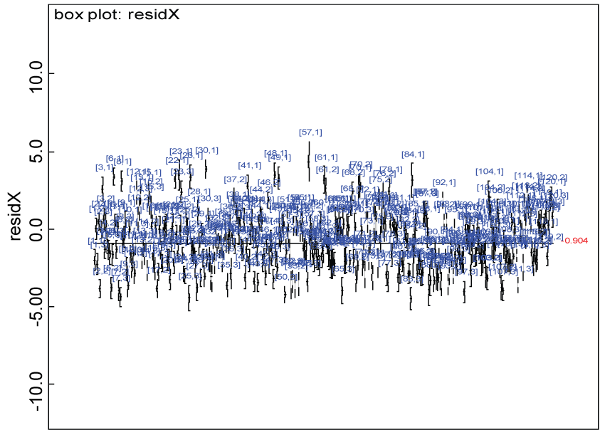Figure 25: Residual plot for domain X for the real data with Cronbach's alpha < 0.7. View Figure 25

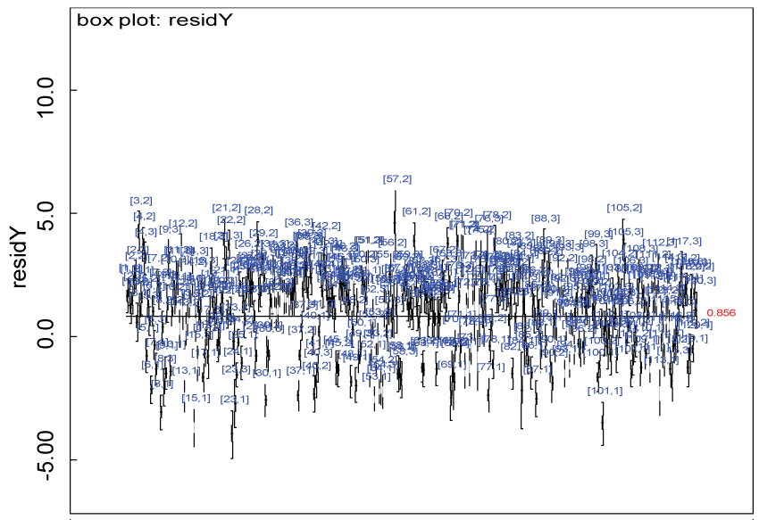Figure 26: Residual plot for domain Y for the real data with Cronbach's alpha < 0.7. View Figure 26

Under the alternative hypothesis: significant treatment effect and homogeneity across the domain

We use a dataset randomly generated to evaluate the model performance under the scenario of alternative hypothesis with homogeneity. The convergence of the MCMC samples for the model parameters is acceptable based on the trace history, autocorrelation and background diagnosis plots. The posterior distributions of model parameters are summarized in figure 8. Per the residual plots in figures 9 and figure 10, for each domain, the residuals for each subject and item fall around the zero line and vary roughly between -5 and 5. This indicates that the model has adequate prediction ability, and that the predicted posterior means can be used to impute missing values. Further, inference on treatment effect within each domain was made based on the posterior distribution of mean scores per treatment group. Box plots as in figure 11, figure 12, and figure 13 are used to demonstrate the posterior distributions of mean scores in each domain and overall. As shown in figures 11, figure 12, and figure 13, there is significant treatment effect in each domain and overall. These results agree with the ones by ANOVA. These observations were further corroborated by simulation studies (N = 1000; > 95% times of significant difference).

Figure 27: Posterior distributions of treatment effects for the two groups within domain X. View Figure 27

Figure 28: Posterior distributions of treatment effects for the two groups within domain Y. View Figure 28

Under the alternative hypothesis: significant treatment effect and heterogeneity across the domain

We use a dataset randomly generated to evaluate the model performance under the scenario of heterogenic alternative hypothesis. The convergence of the MCMC samples for the model parameters is acceptable based on the trace, history, autocorrelation and background diagnosis plots. The posterior distributions of model parameters are summarized in figure 14. Per the residual plots in figure 15 and figure 16, for each domain, the residuals for each subject and item fall around the zero line and vary roughly between -5 and 5. This indicates that the model has adequate prediction ability and that the predicted posterior means can be used to impute missing values. Further, inference on treatment effect within each domain was made based on the posterior distribution of mean scores per treatment group. Box plots as in figure 17, figure 18, and figure 19 are used to demonstrate the posterior distributions of mean scores in each domain and overall. As shown in figure 17, figure 18, and figure 19, there is significant treatment effect in each domain and overall. These results agree with the ones by ANOVA. These observations were further corroborated by simulation studies (N = 1000; > 95% times of significant difference).

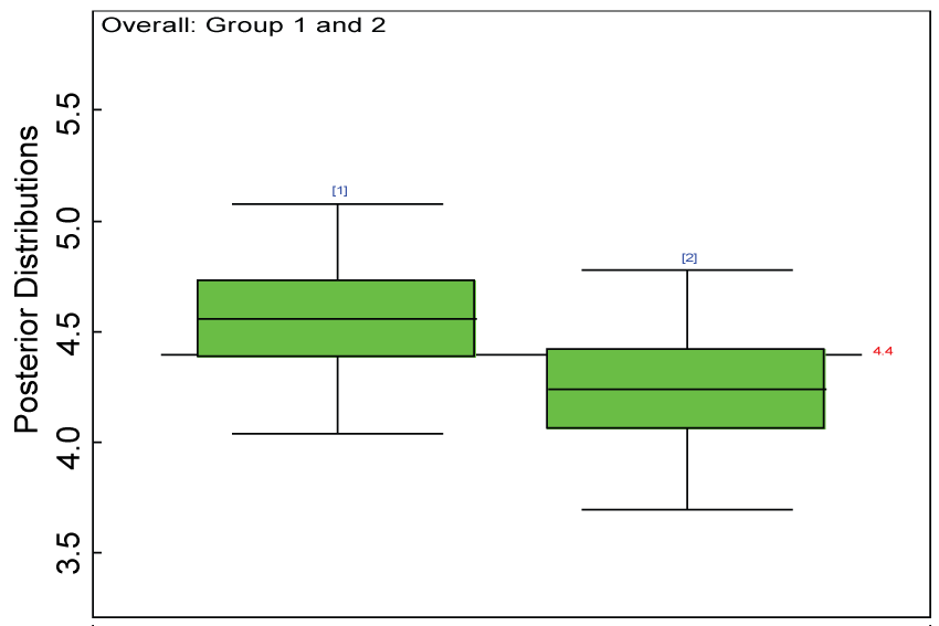Figure 29: Posterior distributions of overall treatment effects for the two groups. View Figure 29

Sensitivity Analyses

We re-parameterized the model including the sensitivity parameter (Δ) that measures departures from MAR. The model parameters for the partially observed data (i.e., parameter vector alpha2 in figure 20) were parameterized as with certain departures from the ones for the completely observed data (i.e., parameter vector alpha in figure 21).

As shown in figures 20 and figure 21, the posterior distributions of model parameters under either the MAR or MNAR assumptions are comparable. With respect to the inferences on treatment effects under the MNAR assumption, the posterior distributions of treatment effects per domain and overall are summarized as in figure 22, figure 23 and figure 24. The treatment effects are comparable to the corresponding ones under the MAR assumptions figure 17, figure 18 and figure 19 but with slightly larger variations.

Real Data Analyses

Our proposed approach are further evaluated using the dataset reported by Jouvent, et al. [13] which includes observations on poly-dimensional rating scale of depressive mode of 20 items from 269 subjects. Since there are no missing values in the data frame, the data are manipulated as described before. The predictive ability of the Bayesian hierarchical model is evaluated based on the residuals defined earlier. The residual plots in figure 25 and figure 26 show that the residuals for both the domain X and Y vary around 0 and range mainly from -5 to 5. The predictive ability of the hierarchical Bayes model is warranted. Inferences on the overall treatment effect and the one within each domain are also performed based on the data with missing values imputed. The posterior distribution of the sum of item scores for each domain (i.e., treatment effect) is summarized and compared between the specified groups as in figure 27 and figure 28. There is no significant difference between the two groups within each domain. Similar results for the posterior distribution of the overall average of the sum of item scores (i.e., overall treatment effect) is given in figure 29.

Discussion

We demonstrated that the multi-level score-type data with missingness can be effectively analyzed using the hierarchical Bayes model with OpenBUGS (Version 3.2.3). In general, such models provide a promising alternative to the conventional approach in dealing with the missingness at the item level particularly when the consistency across the items is not adequate. Even though the conventional approach may be favorable given adequate consistency across the items [14], but it cannot deal with the inherent uncertainty of imputations themselves [15]. The inference based on the proposed model is robust with the non-informative priors. The posterior distributions of model parameters of interest at multiple levels provide more information than do the maximum likelihood estimators (MLEs) even if the computation of MLEs is feasible. The proposed approach can perform well under MAR, particularly when the factors that influence missingness are included in the model. This leads to valid inference based on imputed items. This feature mirrors the merits of regression imputation [15]. However, it is beneficial to perform sensitivity analyses to warrant the validity of the analyses under the MAR assumption.

The proposed method is developed under the cross-sectional setting. When borrowing information across longitudinal observations within a subject is not feasible, it is an efficient way to handle missing values via borrowing information across domains (i.e., scales) and/or borrowing among subjects. Even though this method can ignore the domain structure, it does have the advantage in making good use of domain structure to handle missing data and make inferences at the domain or item level. It makes this approach more appealing than other analogues. In addition, this method can be further extended to the longitudinal setting. Moreover, the distribution of item scores can be ordinal rather than continuous.

As an alternative, the imputed value can be sampled via the following distribution [16]. $Y (X) . u n c u t_{i j} | Z_{i} \sim N o r m a l (Y (X) P_{i j}, σ_{k}^{2})$

This approach is similar to stochastic regression imputation [15], which adds additional noise to the predicted values for imputation. Even though this approach makes sampled values for imputation from the intended distribution, it also causes problems such as implausible/out-of-range values. Therefore, the imputed value needs to be restricted to the range of the item score to assist with convergence. In addition, the feedback of the imputed value may be undesirable and should be avoided via cut function in OpenBUGS. To these aims, we use the following manipulation, $Y (X) . t e m p_{i j} < - c u t (Y (X) . u n c u t i j)$ $Y (X) . t e m p b_{i j} < - a b s (Y (X) . t e m p i j)$ $Y {(X)}_{i j} < - \min (U B, Y (X) . t e m p b i j)$

Here UB is the upper bound of the range of the item scores. This method yields comparable results as the proposed approach.

In the real situations, it is quite often that we encounter with a large number of items, in such situations our proposed approach may not be applicable directly. However, we can reduce the dimension of the items via grouping sets of items and replacing them with their sum scores. But one should be careful in taking this action because it requires that the items are similar enough. Alternatively, we can select a certain number of informative predictors [17].

Conclusions

The proposed hierarchical Bayes model can be used to handle missing data at item level and can help make valid inferences at multiple levels of interest via conditional posterior distributions. It can serve as an alternative to the traditional approach in either the primary or the sensitivity analysis. This approach has the potential to be further extended to other more complicated setting.