We propose to approximate a model for repeated measures that incorporated random effects, correlated stochastic process and measurements error. The stochastic process used in this paper is the Integrated Ornstein-Uhlenbeck (IOU) process. We consider a Bayesian approach which is motivated by the complexity of the model, thus, we propose to approximate the IOU stochastic process into a continuous spatial model that constructed by convolving a very simple and independent, process with a kernel function. The goal of this approximation is to offer some advantages over specification through a spatial process of computing covariance, variogram, and extremal coefficient functions, also to add to the extremal coefficient plots the empirical estimates. This approximation is attractive because it facilitates calculations especially that contain a huge amount of data in addition it reduces the computational execution time, also it extends beyond simple stationary models.
Stochastic process, Longitudinal, Integrated ornstein-uhlenbeck, Bayesian, Spatial, Convolution
62M05, 62M30, 62P10
A longitudinal data consists of measurements of a single variable taken repeatedly over time from an individual. Any approach used to analyze such data must properly consider the correlations among the observations, see Li, N., et al. [1]. The typical structure of longitudinal data is numerous measurements of a possible multivariate response variable on each subject. There could also be covariates, possibly time varying, that influence the response variable [2]. The aim in the analysis of such data is to understand the changes in the mean structure of the response variable with time, to understand the effect of the covariates on the response variable, and to understand the within subject correlation structure.
Let be the longitudinal process of subject at time . Values of are measured intermittently at some set of times . The observed longitudinal data on subject may be subject to "error", thus we observed only whose elements may not exactly equal the corresponding . Given a specification for , the observed longitudinal data are taken to follow
Where is an intra subject error.
In this paper, following Taylor, et al., Xu and Zeger, Wang and Taylor, and Abu Bakar, et al. [3-6] we consider a model of the form
With the notations (N) denotes for Normal Distribution, and denotes for Multivariate Normal with dimension . denotes the observed value of a continuous time-dependent covariates (disease marker or longitudinal measurements) for subject at number of the subjects in the study; number of repeated measurements for subject i and may be different for each subject, is the true value of the marker at time , are independent random intercept of subject follow the normal distribution with mean and variance is fixed slope, is the covariates for subject at time with corresponding unknown regression parameter represents deviations due to measurement error and "local" biological variation that is on a sufficiently short time scale that may be taken independent across j, and is a vector of independent IOU stochastic process, the covariance matrix with parameters and ; only depends on through the number of observations and through the time points at which measurements are taken, see Henderson, Diggle and Dobson [7].
In this paper, we introduce an approximation of the IOU process which still gives an efficient inference of model parameters and reducing the dimensionality and complexity of the model. The details of this simple approach are given in the following sections, including an approximate formulation, the likelihood and parameter estimations. The usefulness of this modeling approach is then demonstrated by simulations.
The main disadvantage of the IOU process is that it is not stationary; hence it is necessary to have a natural time zero for each individual. In some applications, it may be that there is no natural time zero, or that time zero is not exactly known. Large Longitudinal datasets are often defined on naturally heterogeneous fields or have other inherently spatially varying conditions. Therefore, it is unreasonable to expect a response variable to be well-modeled by a stationary process over a large domain space. However, using non-stationary models is difficult in practice due to the conceptual challenges in specifying the model and the computational challenges of fitting the model when the data is so large that memory constraint prevent formation of the covariance matrix.
We propose to approximate the IOU stochastic process into flexible spatial model that can be constructed by convolving a very simple and independent, process with a kernel function. This approximation for constructing a spatial process introduces a number of advantages over specification through a spatial covariogram. In particular, this process convolution specification leads to computational simplifications and easily extends beyond simple stationary models. Our modeling approach is similar to that in Higdon [8], provide simple representations of such model by convolving continuous white noise with a kernel, whose shape determines the covariance structure of the resulting process. This approach is an alternative to traditional geostatistical techniques, where a covariance function is specified directly, but allows for increased flexibility, since the choice of the kernel also allows for features such as non-stationary, anisotropy, and edge effects. Moreover, model (1.2) is temporal longitudinal model, by applying the proposed approximation, the dimensionality of the complex temporal process significantly reduced.
The model we propose for at time is
Where U is a mean zero Gaussian process, and is an approximation of the IOU stochastic process W. Hence, model in (1.2) becomes
But rather than specify through its covariance function, it is determined by the latent process and the smoothing kernel .The restriction on the latent process to be nonzero at the spatial sites in a space time t and define . Each is then modeled as independent draws from a mean zero Gaussian distribution with variance .
Hence, will follow a multivariate normal with mean zero and variance covariance matrix , here is the number of space times over spatial sites .
The new Gaussian process is then
Where is a kernel centered at .
The resulting covariance function for depends only on the displacement vector d = t − s and is given by
Table 1 shows kernels that give standard Gaussian, exponential, and spherical covariograms for the process , [9]. In addition, the covariogram induced by the biwieght kernel Cleveland [10] is also shown.
Table 1: Various kernels and their induced covariance functions in the two-dimensional plane. View Table 1
The process convolution approach gives an approach to build dependent spatial processes, see Ver Hoef and Barry [11]. The basic idea is to build processes that share part of a common latent process in their construction. Perhaps the biggest attraction to these process convolution models is that they give a framework for developing new classes of space and space-time models that allow for more realistic space-time dependence while maintaining some analytic tractability. Generally, one can construct a space-time process by first defining a simple, possibly discrete, process over space and time, and then smoothing it out with one or more kernels, giving a smooth process over space and time.
This constructive approach is appealing since the resulting models can be extended to allow for generalizations such as non-stationarity, non-Gaussian models, and non-separable space-time dependence structures. See Wolpert and Ickstadt [12], and Higdon, et al. [13] for some purely spatial applications, and Higdon [14] for a space-time model. In addition, models can be constructed in such a way to facilitate computation - such as restricting the underlying process to reside on a lattice so that fast Fourier transforms can be employed.
Based upon our previous assumptions, the unknown parameters in model (2.1) are
. The contribution of subject to the conditional likelihood function is given by
Where, and denote marginal and conditional densities, respectively, denotes all model unknown parameters.
For the prior density of we assume tha have independent prior densities, so that are independent and normally distributed with parameters and , also are independent stochastic process with parameter .
From the independency assumptions, the posterior density of all unknown model parameters is proportional of
To fit the full model and make inference about the population parameters, Adaptive Rejection Metropolis Sampling (ARMS), and Gibbs and ARMS sampling techniques are used. These methods are a MCMC technique for drawing dependent samples from complex high dimensional distributions, see Waezizadeh, and Mehrpooya [15]. The posterior distribution converges was checked by Gelman-Rubin convergence statistic R (posterior consistency), as modified by Brooks and Gelman [16]. In order to apply one of these methods on our model, posterior for each parameter must be derived, and then a proposed prior density for each of these parameters must be chosen. Based on the likelihood functions in (3.1) and (3.2), with the notations (IG) denotes for Inverse Gamma, and (N) denotes for Normal, the conditional densities of the unknown model parameters are given as follows:
For the error parameter
Where
, and
In the same manner we found:
The intercept variance , where , and
The intercept mean , where , and
The random intercept , for , where
The average rate of the slope , where
The effect of the regression parameter on the marker , where
-l
and are the remaining covariates after covariate is excluded from .
For the stochastic process parameter , where
, and , , , and is given in (2.2).
Since all posterior densities are in standard form, then it is easy to choose conjugate priors for all model (2.1) parameters, drawing random variates using Gibbs sampler from their full conditional distributions is straightforward since their full conditional densities are standard distributions. Therefore, we use the full conditional density as proposal density. At each updating step for these parameters, a new draw from the full conditional density is always accepted.
To illustrate our proposed model, we setup our simulation study represents a randomize clinical trial, in which M = 500 subjects are randomized. Each longitudinal marker in model (2.1), , was simulated as the sum of the trajectory function and the error terms , each subject has its observed longitudinal measured at time points . For the simulations considered in this research the smoothing kernel will be a radially symmetric kernel, such that , with variance covariance function , and defining the latent process support so that the are m = 5 equally spaced points ranging from -0.1 to 1.2. Note that this combination of kernel width and spacing of the yields a spatial process via (2.3) that is nearly stationary. If the spacing become much larger, or if the kernel width is reduced, the covariance structure for becomes unduly influenced by sparseness artifacts.
Since the calculations for the simulation study were highly computationally intensive, we have used the cluster with about 20 nodes with AMD Quad-Core Opteron 835X, 4 × 2G Hz, and 16 GB RAM per node. We obtained 3000 iterations after a burn-in of 1000 iterations. Convergence was checked by monitoring histories of sampled quantities with several different starting points. The histogram, the time series plots of one sequence of Gibbs samples for different number of iterations and the average number of these iterations for the parameter are presented in Figure 1.
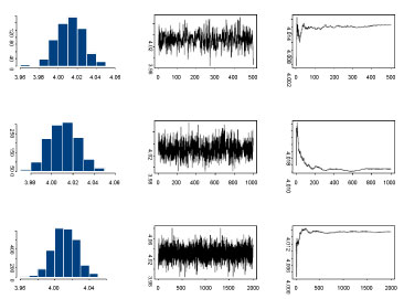 Figure 1: Histogram, time series and average values plots respectively for the parameter values μa at 500, 1000, and 2000 iterations respectively, using Gibbs sampler. View Figure 1
We also used the Gelman-Rubin convergence statistic, as modified by Brooks and Gelman [15]. They emphasize that one should be concerned both with convergence of R is the ratio pooled-width within-width (the ratio of width of the central 80% interval based on pooled runs and the average width of 80% intervals within the individual runs), to one, and with convergence of both the pooled and within interval widths to stability. For our analyses, all R's converged to 1 within 3000 iterations and hence the burn-in of 1000. The analysis for the 500 simulated data sets for a single scenario took approximately 2:30 hours to run the model under the approximate model. While it took almost 6 hours to run the analysis without approximations.
With the initial values of the parameters for which the data are generated considered as the truth values of the parameters, estimate Monte Carlo Summary statistics, Monte Carlo Standard Deviation (MCSD), Mean Squared Error (MSE), 95% Confidence Converge Rate (CCR), and Bias in Percentage Terms (BPT) are presented in Table 2, where, MCE stand for Monte Carlo Error and it can be evaluated as follows : In our simulate study we used 500 data replications, thus the resulting estimates are subject to sampling variation (Monte Carlo Error), this variation for the point estimate can be calculated as , the MCE then can be found by
Table 2: Monte Carlo Summary statistics of the parameter estimates. View Table 2
Results in Table 2 assert the convergence of the Markov Chain and the samplers reached the convergence after 2,000 iterations after 1,000 iterations are burn-in. Posterior means, posterior standard deviations, Bias as percent of true parameter and 95% highest posterior density intervals for each parameter in the proposed and IOU models, are represented in Table 3. The estimates of all parameters from the approximate modelling analysis are quite accurate and efficient.
Table 3: Posterior estimates from proposed and IOU models. View Table 3
We have proposed a new model for repeated measures that incorporated random effects, correlated stochastic process and measurements error, we proposed to approximate the IOU stochastic process into a spatial model that can be constructed by convolving a very simple and independent, process with a kernel function. This approach offered some advantages over specification through a spatial process of computing covariance, variogram, and extremal coefficient functions, also added to the extremal coefficient plots the empirical estimates. This approximation is attractive because it facilitates calculations, especially that contain a huge amount of data also it easily extends beyond simple stationary flexible models. Moreover, this structure can be used to significantly reduce the dimensionality of a complex temporal process.
The limitation in the proposed model is that the latent process must be nonzero at the spatial sites in a space time t. To overcome this problem with the covariance function of and the differences through the displacement vector d = t – s was performed.
A Bayesian approach was taken to fit the proposed model through a simulation study. The numerical results demonstrate that the propose modelling method results in efficient estimates and good coverage for the population parameters. The estimates are close to the true values of the parameters and have good coverage rates. The small biases of the estimates are due to Monte Carlo simulation error. Compared to the IOU model, the proposed model results in improved estimates almost for all parameters. The proposed model demonstrated significant reductions in execution time. This approach effectively eliminates the deficiency of non-spatial huge data access by replacing such patterns in hotspots of applications with spatial sites data at a space time t at runtime. The execution time reduced by 60% illustrate the efficiency of proposed model.