An in-depth study using the database from GLOBOCAN, CDC, and WHO health repository highlights the lethality of breast cancer, taking thousands of lives each year. Therefore, timely prediction of cancer can help patients to consult the doctor on time. In the past various studies have successfully predicted the nature of the tumor to be benign or malignant and if the breast cancer tumor will reoccur or not. However, no time-based models have been studied previously. With the help of Machine Learning, this study has shown various prediction models that can predict the time as accurately as 1 year for the tumor to reappear in malignant patients. In this prediction analysis performed on the 198 patients, 40% of the total patients were predicted to have breast cancer tumors reoccurring within 1st year of the diagnosis. The proposed machine learning techniques use various classification models such as Spectral clustering, DBSCAN, and k-means along with prediction models like Support Vector Machines (SVM), Decision trees, and Random forest. The results demonstrate the ability of the model to predict the time taken by the tumor to reoccur or the time taken by the patient for full recovery with the best accuracy of 78.7% using SVM. This population-based study performed on multivariate real attributed characteristics data can therefore provide the patients a reasonable estimate about their recovery time or the time before which they should consult the doctor.
Breast cancer, Machine learning, Prediction model
According to the report [1] of the Centers for Disease Control and Prevention (CDC), breast cancer is one of the most common cancers among women. About 10% to 15% of all the worldwide women develop the disease in their lifetime [2]. As per the data reported by CancerStats-UK, every year over 44,000 women develop the disease, and more than 12,500 die from it within the United Kingdom (UK) [3]. In 2017, within the USA every 125 per 100,000 women were diagnosed with breast cancer accounting for a total of 250,520 new cases and 42,000 deaths being reported [4]. National Cancer Registry Program and International Agency for Research on Cancer have identified breast cancer as the most common cancer among women in India, accounting for 14% of all the cancers in women [5,6]. In 2018, there were 162,468 new cases and 87,090 deaths reported in India with 1 in 22 urban women and 1 in 60 rural women likely to develop breast cancer during their lifetime [7].
In 2020, a study [8] conducted by World Health Organization (WHO) showed that over 2,000,000 new cases and over 600,000 deaths were reported due to breast cancer in a single year. Figure 1 shows the summary of the reported data where it can be seen that cancer has affected women around the globe. Eastern Asia tops the list and accounts for 551,636 of the total new cases with North America, South-Central Asia, and Western Europe following it with 281,591 new cases, 254,881 new cases and 169,016 new cases reported respectively. Eastern Asia also tops the list for a total number of deaths, accounting for 141,421 deaths with South-Central Asia, South-East Asia, and Central & Eastern Europe following it with 124,975 deaths, 58,670 deaths, and 51,488 deaths reported, respectively. Previous studies [9] show that various cancers share hormonal and epidemiological risk factors and a woman with breast cancer is also likely to have a risk of developing ovarian or endometrial cancer. Due to this reason, the treatment of breast cancer becomes complicated. For instance, Visvanathan K, et al. [10] reported that tamoxifen can be used for breast cancer prevention but Vogel VG, et al. [11] showed that Tamoxifen also increases the risk of endometrial cancer.
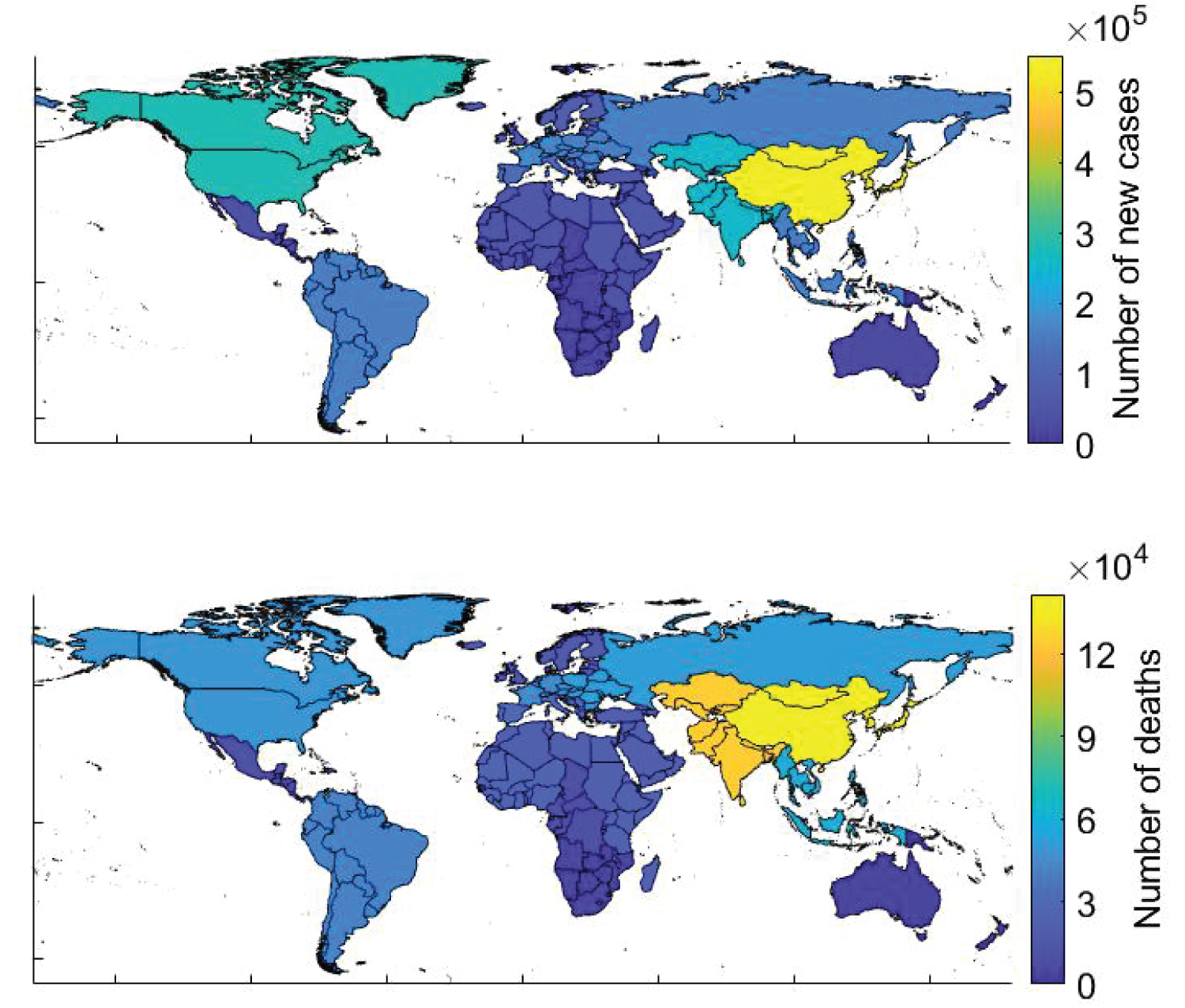 Figure 1: New breast cancer cases and deaths as reported by WHO in 2020.
View Figure 1
Figure 1: New breast cancer cases and deaths as reported by WHO in 2020.
View Figure 1
Early diagnosis and prediction of breast cancer can therefore improve the chances of survival as it can promote timely clinical treatments to the patients. Apart from this, having a pre-hand knowledge of breast cancer might influence a women's decision regarding taking a certain medical drug for breast cancer prevention that can increase the risk of another type of cancer. Early prediction of breast cancer or time of recurrence can encourage screening for high-risk women and promote adherence to screening guidelines. Besides, it can also recommend chemoprevention and other suitable actions to reduce one's risk [12,13].
Machine learning is a combination of tools and methods that can be used to create algorithms that can help in prediction, classification, and pattern recognition. One of the advantages of using machine learning models over statistical models is the amount of flexibility in capturing high-order interactions between the data, which might result in better predictions [14]. The use of machine learning in predicting breast cancer has been widely studied over the decades. In the past various machine learning and data mining techniques have been used to predict and classify breast cancer. Quinlan JR [15] in 1996 studied 10-fold cross-validation with the C4.5 decision tree method and showed a benign and malignant classification accuracy of 94.74%. In 1999, Pena-Reyes CA and Sipper M [16] introduced a combination of fuzzy genetic approach and evolutionary algorithm to automatically produce a diagnostic system with a classification accuracy of 97.36%. Setiono R [17] in 2000 demonstrated the 98.10% accurate classification based on feed-forward neural network rule extraction algorithm. Zhou Z and Jiang Y [18] used the C4.5 method along with Artificial Neural Networks on 683 record UCI machine learning datasets to classify tumors into benign and malignant. Delen D, et al. [19] used decision trees on the SEER (1973-2000) dataset to predict survival and deaths of patients. Al-Hadidi MR, et al. [20] demonstrated supervised learning and compared Back Propagation Neural Network and Logistic regression models. Jivani AG, et al. [21] compared the performance of decision tree, Bayes classification, and K-nearest neighbor algorithm. Osman AH [22] combined a two-step clustering technique with a support vector machine to enhance the classification problem. Akay MF, [23] introduced the use of a Support Vector Machine combined with feature extraction. Zheng B, et al. [24] investigated feature extraction using a hybrid K-means and support vector machine algorithm. Chaurasia V and Pal S [7] compared the performance of various supervised learning classifiers such as Naïve Bayes, Support Vector Machine, and Decision tree on various breast cancer datasets.
This paper takes into account three different methods namely Spectral clustering, DBSCAN, and k-Nearest neighbors to cluster and classify the tumor as benign and malignant. Although the use of machine learning in breast cancer prediction has been extensively investigated but there is no study that focuses on the prediction of the time of full treatment or time of tumor recurrence in the patient's body. This paper lays down the foundation of how various techniques like Support Vector Machines, Decision trees, and Random forest can be used to predict the patient's treatment time in a yearly manner. All three methods are shown to have the capability of predicting the treatment time between less than 1 year to 11 years. This prediction can lead to patients' timely treatment and consultation with the doctor in turn saving their life.
For accurate prediction, diagnostic and prognostic datasets are considered separately. The prognostic dataset is trained for classifying and predicting the recurring and full treatment cases. This prediction model is then used on the malignant cases obtained from the diagnostic dataset to predict if the tumor is recurring or nonrecurring in the patient's body. Each of these cases is then evaluated to predict the time taken by the tumor to reoccur or the time taken by the patient for full treatment. The workflow has been summarized in Figure 2.
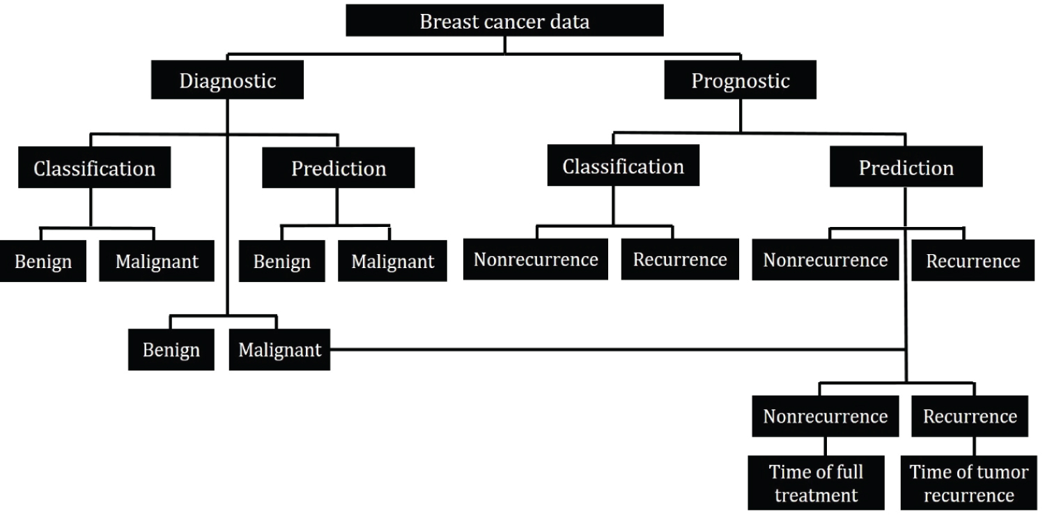 Figure 2: Workflow schematic.
View Figure 2
Figure 2: Workflow schematic.
View Figure 2
The multivariate real attributed characteristics data [25] is taken from the University of California Irvine's Machine Learning Repository (UCI). The data was collected by Dr. Wolberg WH at the General Surgery Department of Clinical Science Center at the University of Wisconsin Madison and was donated to UCI by Street N. Two different datasets are considered in this study. I) Wisconsin Diagnostic Breast Cancer data (WDBC) and II) Wisconsin Prognostic Breast Cancer data (WPBC). A digitized image of a fine needle aspirate (FNA) of a breast mass was used to obtain characteristics of cell nuclei present in the image and 30 different features were calculated for each patient. The WDBC and WPBC are 30 features datasets of 569 patients and 196 patients respectively. In addition to the feature values, the dataset also consists of the corresponding labels i.e. Benign (B) and Malignant (M) for WDBC and Recurring (R) and Nonrecurring (N) for WPBC data. The data has been summarized in Figure 3 and the mean values of the data are reported in Table 1.
 Figure 3: Data summary. a) Wisconsin Diagnostic Breast Cancer (WDBC) data; b) Wisconsin Prognostic Breast Cancer (WPBC) data.
View Figure 3
Figure 3: Data summary. a) Wisconsin Diagnostic Breast Cancer (WDBC) data; b) Wisconsin Prognostic Breast Cancer (WPBC) data.
View Figure 3
Table 1: Mean value of features. View Table 1
To ensure a good quality of the sampled data, all the benign and malignant cases obtained using FNA were confirmed by surgical biopsy [26]. In addition, the use of Xcyt software for breast mass image analysis was also verified on 131 new diagnosed cases (94 B, 37 M) with 100% accuracy [26,27].
k-means clustering: k-means is an unsupervised, iterative learning and data partitioning algorithm that minimizes the within-cluster sum of squared distances from the cluster mean [28]. This algorithm assigns k clusters to n observations by centroids, where k ≤ n. The algorithm can be written mathematically as shown in Equation 1 [29].
where i is the index of the variable x which belongs to the set and S is the set in which the data is partitioned, with k being the total number of classification sets. In addition, is the mean of the points in S1.
Equation 1 can be further simplified and written to minimize the pairwise squared deviations of points in the same cluster. This is described in Equation 2 [29].
This equivalence relation is deduced using the identity shown in Equation 3.
Density-Based Spatial Clustering of Application with Noise (DBSCAN): DBSCAN is a density-based clustering algorithm developed in 1996, which aims to cluster the data in arbitrary shape based on the density of data points in an area [30]. This can be mathematically represented by the definitions (a), (b), and (c) posed by Ester M, Kriegel HP, et al. [31]
(a) ∀ p, q: if p ∈ C and q is density-reachable from p concerning Eps and MinPts, then q ∈ C.
(b) ∀ p, q ∈ C: p is the density - connected to q with respect to Eps and MinPts
(c) N = {p ∈ D| ∀ i:p ∉ C } i.e. noise (N) is the set of points in the database D not belonging to any cluster C
Where D is the database of points, C is the cluster, Eps stands for epsilon neighborhood of a point specified as a numeric scaler that defines a neighborhood search radius around a point and MinPts stands for the minimum number of points required to form a dense region. In addition, p and q are any two random points taken arbitrarily.
Therefore, with a given value of Eps and MinPts, a cluster can be obtained first by choosing an arbitrary point from the dataset and then retrieving all the points that are density-reachable from the chosen point [31].
Spectral clustering: Spectral clustering is a graph-based algorithm that uses the data's spectrum of similarity matrix to perform dimensionality reduction (M to M' where M' < < M) before clustering the data in fewer dimensions [32]. This is advantageous because, with fewer dimensions, clusters in the data can be more widely separated. The new set of reduced dimensions is obtained using the eigenvectors of a Laplacian matrix, which is one of the many ways to represent a similarity graph that can model the local neighborhood relationships between data points [33]. Assuming that the data consist of n points x1, x2, x3, ....xn, pairwise similarities can be written as sij = s(xi,xj) by using some similarity function which is symmetric and non-negative. The corresponding similarity matrices [34] can then be obtained as S = (Sij)i,j = 1...n. The working of the algorithm was demonstrated by Luxburg UV, et al. [35] using the mathematical conditions (a) or (b) and (c) for a given similarity matrix S.
(a) (for unnormalized spectral clustering)
(b) (for normalized spectral clustering)
(c) where A and are two mutually exclusive clusters
where, for unnormalized spectral clustering, the graph Laplacian is defined using Equation 4 with D as the diagonal matrix having entries
L = D - S # (4)
and for normalized spectral clustering, the graph Laplacian is defined by equation 5
L'' = D-1L = I - D-1K # (5)
This Laplacian graph matrix can therefore be used to get the new eigenvector thereby providing the reduced dimensions.
Support vector machines: Support vector machines (SVM) is a supervised learning algorithm that can help analyze the data by classification and regression analysis. In addition, it is a Neural Network system that can achieve higher generalization performance as compared to traditional neural networks [36]. One of the main advantages of using SVM over other neural networks is that training SVM is equivalent to solving linearly constrained quadratic programming problems, which ensures that the solution is always unique and globally optimal [37]. The working of the SVM is related to forming a hyperplane, which can maximize the margin by diving the data into different classes where the margin refers to the nearest distance from the hyperplane to the point of each class [38]. The working of the algorithm can be represented mathematically by using conditions [39] (a) and (b) for a given dataset
(a)
(b)
where maps xu into higher dimensional space and K > 0 is the regularization parameter.
There are several methods to deploy SVM, but in this manuscript, the LIBSVM support library has been considered. The use of this library enables the algorithm to get trained on a given dataset and obtain an SVM model, which can then predict information on a testing dataset [40].
Decision trees: Decision trees are recursive structures and sequential models, which use logic to combine different sequences of simple tests. They use a threshold value against each test to compare a numerical attribute [41]. The decision-making process starts at the root node of the tree and is continued using the appropriate subtree until a leaf (last node) is encountered. Upon reaching the last node, a final decision is made giving out the label which can then be used to predict the class [42]. The schematic is shown in Figure S1a. Quinlan JR [43] laid down the method for creating the decision tree for m classes denoted by {C1, C2, C3, ..... Cm} and training set, T. This has been paraphrased using statements (a), (b) and (c) [42].
(a) The decision tree is a leaf identifying class Ci if T contains one or more objects belonging to a single class Ci
(b) The decision tree is a leaf determined from information other than T if T contains no objects
(c) If T is a set of a mixture of classes, then based on a single attribute, a test is chosen that has one or more mutually exclusive outcomes {O1, O2, O3 ... On}, where n is the total number of outcomes. T is partitioned into subsets T1, T2, T3, .... Tn where Tj contains all the objects in T that corresponds to the outcome Oj of the chosen set. This step is then repeated to each subset of training objects.
Random forest: Random forest is an algorithm that combines classifiers based on decision trees. Unlike decision trees, in Random forest, the trees are not associated among themselves. The main goal behind this algorithm is to build N decision trees to obtain N training sets. The forest can be grown based on the number of trees defined by the user and holds the advantage of having high variance and low bias [44]. This algorithm works by randomizing the dataset to form different decision trees and labeling the outcomes. The outcomes of each decision tree are treated as votes and the majority vote is used to assign the final label to the data instance. The schematic is shown in Figure S1b. The algorithm can be mathematically written using the statements (a) and (b) [45].
(a)
(b)
where f(u,vi), i = 1,2,....i, is a set of decision trees with u as the input and v as the label vector. X and Y are randomly generated vectors from the dataset. mg is the margin function, av is the average, I is the indicator function, P is the probability and φ is the generalization error. In statement (a), fi(X) = Y is the result of classification and fi(X) = i is the result of classification with i. The margin measures the extent to which the average number of votes at X, Y for the correct class exceeds the average vote for any other class [44].
One of the major objectives of this study is to classify the data as benign/malignant and recurring/nonrecurring. Three different clustering methods namely k-means clustering, Density-based Spatial Clustering of Application with Noise (DBSCAN) and Spectral clustering (SC) are used. The accuracy and the classification are obtained by developing a confusion matrix as shown in Figure S3.
The diagnostic dataset (WDBC) lists 569 patients and classifies the tumor as benign or malignant. This study aims to propose an algorithm to predict the nature of tumor occurrence for all the malignant cases and predict the time taken for a full treatment or the time when the tumor reoccurs. The entire prediction process is broken into three steps.
Step 1: The WPBC dataset contains the list of 198 patients along with breast cancer features, occurrence labels, and the time parameter. Figure 4 shows the survival plot corresponding to the WPBC dataset. For all the cases having the label as recurring, the value of time refers to the time taken by the tumor to reoccur back whereas, for all the cases having a label of nonrecurrence, the time value refers to the time taken by the patient for a full recovery. It can be seen from Figure 4a that for more than 70% of the patients marked with recurrence label, it took more than 6 years for the tumor to reappear, whereas more than 70% of patients marked with nonrecurrence label were fully treated within 6 years.
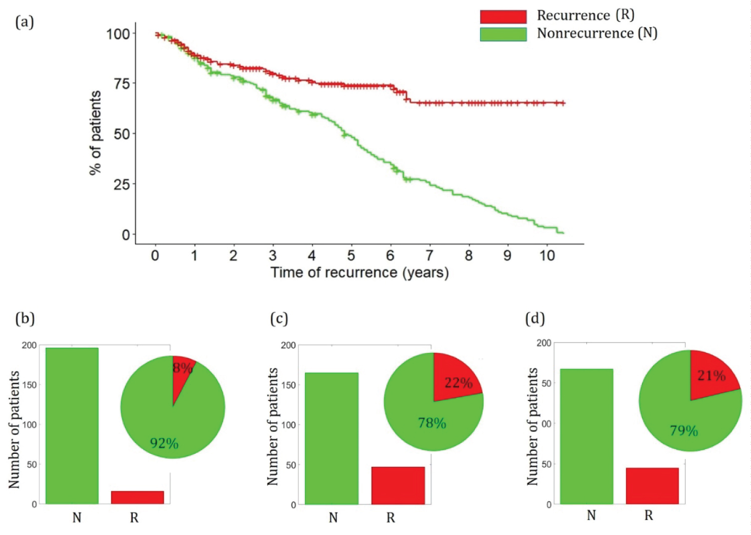 Figure 4: a) Survival plot of WPBC dataset; b) Prediction of WDBC malignant cases into recurring and nonrecurring cases using SVM; c) Decision trees; d) Random forest.
View Figure 4
Figure 4: a) Survival plot of WPBC dataset; b) Prediction of WDBC malignant cases into recurring and nonrecurring cases using SVM; c) Decision trees; d) Random forest.
View Figure 4
The WPBC dataset is trained following 3-fold cross-validation. The importance and schematic of 3 cross-validation is presented in the Supplementary. Three different training methods namely Support Vector Machines (SVM), Decision tree (d-tree), and Random forest (RF) are used to predict the nature of occurrence and classify the malignant WDBC cases as recurring or nonrecurring. The details and the corresponding mathematical representations of the algorithm along with error analysis for all the methods are presented in the Supplementary. Figure 4b, Figure 4c, and Figure 4d show the summary of the predictions made by different algorithms. As can be seen, SVM predicts that 8% of the total 212 malignant WDBC cases are recurring, whereas decision tree and random forest predicts that 22% and 21% of the malignant cases are recurring.
Step 2: After the malignant WDBC cases have been classified as recurring or nonrecurring, the WPBC data is trained to predict the time of treatment/recurrence. This is performed by assigning new labels to the WPBC dataset. The label is assigned 1 if the time length is within the appropriate month range as shown in Table 2. The WPBC dataset is then trained using the time-based labels and the prediction models are obtained.
Table 2: Time-based label assignment. View Table 2
Step 3: The developed prediction models are then used to predict the time for all the malignant cases obtained from the WDBC dataset. If the case is classified as recurring in step 1, then the predicted time will be the time taken for the tumor to reoccur and if the case is classified as nonrecurring in step 1, then the predicted time will be the time taken by the patient for full treatment.
The diagnostic data (WDBC) corresponds to 569 patients with 357 benign and 212 malignant cases. Three different clustering algorithms namely Spectral Cluster, DBSCAN, and k-means are used to partition the data into benign and malignant using all the 30 features. Based on the classification labels, a confusion matrix for each method is obtained along with the accuracy using Equation S1 given in the Supplementary. It can be seen from Figure 5a that the k-means algorithm has the highest accuracy of 85.4%, followed by DBSCAN and Spectral cluster with an accuracy of 82.1% and 47.6% respectively.
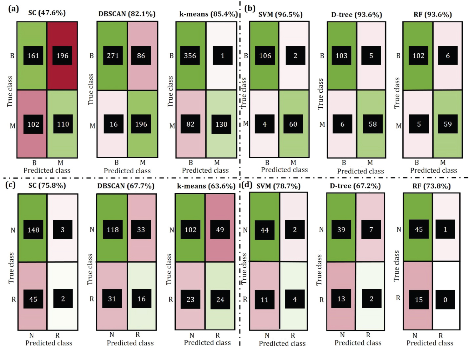 Figure 5: Confusion matrix for clustering and prediction where B = benign and M = malignant, N = nonrecurring and R = recurring. a) Clustering on WDBC; b) Prediction on WPBC; c) Clustering on WDBC; d) Prediction on WPBC.
View Figure 5
Figure 5: Confusion matrix for clustering and prediction where B = benign and M = malignant, N = nonrecurring and R = recurring. a) Clustering on WDBC; b) Prediction on WPBC; c) Clustering on WDBC; d) Prediction on WPBC.
View Figure 5
One of the major objectives of this study is to predict the nature of tumors based on the given features. The entire WDBC dataset is divided into 3 different sets, trained on 2 of them, and tested on the remaining set. This is repeated until all the sets have been tested using the 3-fold cross-validation technique. It can be seen from Figure 5b that SVM is able to predict the nature of the tumor correctly, with 96.5% accuracy whereas Decision tree and Random forest both have an accuracy of 93.6%. The corresponding decision tree and random forest tree diagram are presented in Supplementary (Figure S5 and Figure S6). The accuracy of SVM can be increased further by training more samples in the dataset, this is shown in the Figure S4a. However, an increase in the training dataset will cause a decrease in the validation dataset. To avoid over-fitting or under-fitting the model was trained with a 70/30 ratio for train/validate dataset. For the Random forest algorithm, it can be seen in Figure S4b that out of bag classification error given by PX,Y(mg(X,Y) < 0, decreases as the number of trees in the random forest are increases. In addition, the steady value of error at 0.05 also shows the convergence of the algorithm.
The WPBC dataset corresponds to 198 patients with 151 nonrecurring and 47 recurring cases. It can be seen from Figure 4c that the Spectral-clustering algorithm has the highest accuracy of 75.8%, followed by DBSCAN and k-means with an accuracy of 67.7% and 63.6% respectively.
Prediction of recurrence and nonrecurrence is an important aspect of this study because it is later used to predict the time taken for a full treatment or the time taken for the tumor to reoccur. It can be seen from Figure 4d that SVM can predict the occurrence/nonrecurrence with the accuracy of 78.7% followed by Random forest and Decision tree with 73.8% and 67.2% accuracy respectively. Similar to the prediction in WDBC, the accuracy of SVM increases with an increase in the number of training data. This is shown in Figure S7. The decision tree along with the convergence of random forest is also presented in Figure S8, Figure S9, and Figure S10.
The year-wise tree diagram for Decision tree and Random forest have been provided in Supplementary (Figure S11 - Figure S46).
It can be seen from Figure 6 that all three methods are capable of predicting the time of recurrence/full treatment within a range of 1 to 11 years. SVM predicts that 8 recurring case patients will have tumor reappearing within 1 year while this prediction number is higher for the Decision tree (18 patients) and Random forest (17 patients).
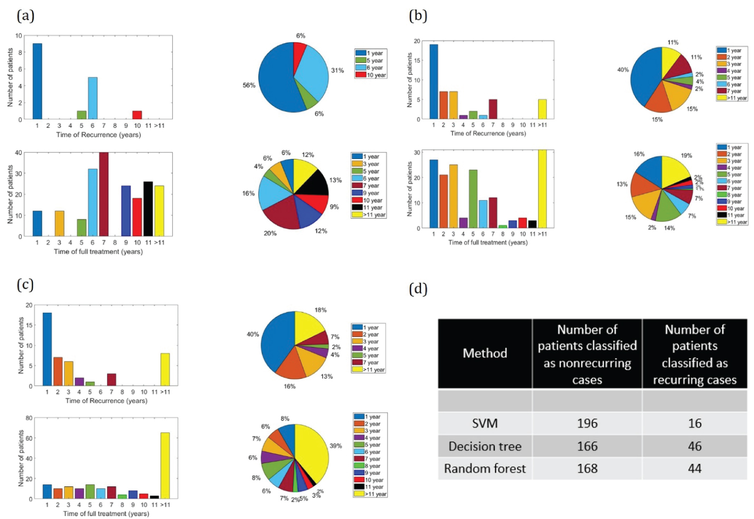 Figure 6: Prediction of time of recurrence/full treatment. a) SVM; b) Decision tree; c) Random forest; d) Number of recurring and nonrecurring cases corresponding to different prediction methods.
View Figure 6
Figure 6: Prediction of time of recurrence/full treatment. a) SVM; b) Decision tree; c) Random forest; d) Number of recurring and nonrecurring cases corresponding to different prediction methods.
View Figure 6
Machine learning and data mining techniques are playing an important role in medical applications. This study investigates the use of the Spectral clustering algorithm, DBSCAN algorithm, and k-means algorithm for clustering the diagnostic data into benign and malignant and prognostic data into a recursive or nonrecursive tumor. The classification accuracy is shown to be as high as 85.4% for Wisconsin Diagnostic Breast Cancer (WDBC) data using the k-means algorithm and as high as 75.8% for Wisconsin Prognostic Breast Cancer (WPBC) data using Spectral clustering. The study proposes Support Vector Machines (SVM), Decision tree, and Random tree algorithm for developing prediction models. These prediction models upon using 3-fold cross-validation show an accuracy of 96.5% on WDBC data and 78.7% on WPBC data using SVM. The WPBC trained prediction models are then used on the WDBC dataset to predict the time taken by the patient for full treatment or time taken by the tumor to reoccur in the body as accurately as 1 year. This work therefore can provide the patients a reasonable estimate about their recovery time or the time before which they should consult the doctor.
While the classification and prediction of tumor (into benign/malignant or recursive/nonrecursive) have been studied over the decade, none of the earlier work demonstrates the prediction of time taken for the full treatment or time for the tumor to reoccur as accurately as this study. Support vector machine is shown to predict that 16% of the total nonrecurring tumor patients will be fully treated within the first 5 years, whereas the Decision tree and Random forest predicts 60% and 35% full treatment within the first 5 years of diagnosis. All three prediction methods are shown to predict that at least 40% of the total malignant tumor patients will have the tumor recurring within 1st year. Having the timely knowledge of the tumor can therefore warn the patients to consult the doctor and start their treatment as soon as possible thus saving many lives.
The author declares that they have no known competing financial interests or personal relationships that could have appeared to influence the work reported in this paper.