The COVID-19 pandemic has revealed facts about deficiencies in health resource planning of some countries having relatively high case count and death toll. The virus has undergone an observed increase of cases that led to a global pandemic. Many authors have developed different models for predicting or observing the current trend of COVID-19 pandemic. In this study, fitting birth and death models using Maximum Likelihood Estimation (MLE) method with application to COVID-19 in sub-Sahara Africa is proposed. Real life data on COVID-19 from World Health Organization (WHO) and other online resources was used to determine probability distributions of infected, recovery and death of COVID-19 patient in some selected Sub-Sahara countries: Nigeria, Kenya, South Africa and Central African Republic (CAR) from inception of the disease to 10th November, 2021. The MLE method was used to determine the probability of getting infected with COVID-19; the probability of having more than n COVID-19 active cases in a susceptible population; the average survival time of the virus in a system; and the average number of COVID-19 active cases per day. The result of the analysis showed that the probability of recovery is above 0.9 for the selected countries except for Central African Republic which is 0.5924 and South Africa has the highest mortality rate of 3.06%. Kenya has the highest probability of having more than 10 COVID-19 cases. Kenya also has the highest survival time for the virus and has the highest number of COVID-19 active cases per day. The results fit well to the case data of the sample corona center. Current preventive and responsive resource planning depends on accurately designed models and methods needed for the prediction of future threats, and mitigation costs.
Birth and death process, COVID-19 pandemic, Maximum likelihood estimation, Simple queuing system, Sub-Sahara African
Accurate modeling of viral outbreaks in living populations is a prominent research field. Many researchers are in search for simple and realistic models to manage preventive resources and implement effective measures against hazardous circumstances. The ongoing COVID-19 pandemic has revealed the fact about deficiencies in health resource planning of some countries having relatively high case count and death toll. In order to sufficiently analyze the transmission and recovery dynamics of epidemics it is important to choose concise mathematical models. Hence, the Birth-Death (BD) process - a stochastic modeling, approach tied to queuing theory has been chosen.
The Birth-Death (BD) process is a special case of continuous-time Markov process where the state transitions are of only two types: "births", which increase the state variable by one and "deaths", which decrease the state by one. The model's name comes from a common application, the use of such models to represent the current size of a population where the transitions are literal births and deaths. Birth-death processes have many applications in demography, queuing theory, performance engineering, epidemiology, biology and other areas. There already an extensive statistical theory for estimating the parameters of queuing models and stationary BD processes; for example, [1-5]. This BD process can also be applied to new cases of COVID-19 and closed cases of COVID-19. The maximum likelihood estimation is used to estimate the parameters of the model. COVID-19 closed cases are the sum of COVID-19 induced deaths and recovered cases. When closed cases are subtracted from infected individuals, what are left are the active cases.
The first case of COVID-19 in SSA was stated on 28 January 2020 in Nigeria [6], which spread to all SSA. In Sub-Sahara Africa, the active cases at present are decreasing as a result of high rate of recovery. As the COVID-19 pandemic spread across the globe in 2020, Sub-Saharan Africa appeared to have been spared the worst: While reported cases and deaths mounted alarmingly in Europe and North and South America, they remained consistently lower on most of the subcontinent, except for South Africa [7]. Some of the predictions proved correct, for instance, the region's relatively young population (only 3% ages 65 and older) may explain why it has reported fewer COVID-19 deaths than other regions. Early May 2021, Sub-Saharan Africa reported 3.2 million accumulative COVID-19 cases and about 83,000 deaths, accounting for about 2% of global cases and deaths, respectively, while representing 14% of the world's population [8].
The COVID-19 new laboratory infected cases can be taken as a birth process while the recovery/death can be taken as the death process. Thus, the BD process is used to model COVID-19 active cases and closed cases.
Numbers of studies have worked on COVID-19 pandemic, particularly in the area of statistical, dynamical and mathematical modelling. [9] worked on mathematical models of COVID-19 dynamics and concluded that the exposure time is a significant factor in spreading the disease with a basic reproduction number of 2, 14-day incubation period, and concluded that if an infected person stay more than 9 hours in the event could infect other people. [7] used hierarchical polynomial regression models to predict transmission of COVID-19 at global level and made a forecast with the model. They concluded that if there is no new phase of the virus and there are compliances to government policies to prevent the spread of COVID-19 as advised by the Centre of Disease Control (CDC) and WHO, then new cases of COVID-19 per day globally would reduce significantly in coming days. [10] adopted three kinds of mathematical models, namely logistic model, Bertalanffy model and Gompertz model and adjourned logistic model the best among the three models studied and used it to predict the number of individuals expected to be infected in Wuhan, non-Hubei province and in the entire China. [11] worked on the dynamic models of the six chambers, and established the time series models based on different mathematical formulas according to the variation law of the original data. They produced results based on time series analysis and kinetic model analysis and used it to predict future spread of the virus.
[12] used models based on multi-dimensional adjustment by means of polynomial equations assuming a linear dependence of the function with respect to each of the variables on which it depends in order to assess the development of epidemics. Adeniyi, et al. [13] developed a dynamic model of COVID-19 disease with exploratory data analysis. Their model assumed that education on the disease transmission and prevention induced behavioural changes in individuals to imbibe good hygiene, thereby reducing the basic reproduction number and disease burden. [14] analyzed COVID-19 pandemic data with visualization and moment about midpoint using exploratory and expository analyses and concluded that average number of COVID-19 new cases and new deaths would decrease in coming months but there will be increase in the cumulative cases and deaths but at a slower rate. [15] also undertook a study to determine the proportion of Nigeria's population that will be prone to the COVID-19 pandemic as well as the proportion of infections, recoveries and fatalities from the COVID-19 pandemic employing a Markov model.
Hence, this study aimed at fitting birth-and-death model to COVID-19 data using maximum likelihood estimation to estimate the parameters of the model. The data are COVID-19 cases of four selected Sub-Sahara African countries Nigeria, Kenya, South Africa and Central African Republic (CAR). The BD model developed for COVID-19 cases will help to determine average time an infected individual will live with the virus before recovery or death. It will also help to know the expected number of active cases in a particular population of interest. Health workers and medical doctors want to know how long COVID-19 infected individuals will have to battle with the virus before the individual recovers or dies. This can be facilitated by medical treatment and the body immune system. If the body immune system is strong the infected individual recovers, but if it is weak, the individual may die. Generally, on the average the waiting time from infection to recovery might not be known and the probability distribution of the waiting time is also unknown. There is no appropriate model predicting the average waiting time between infection and recovery. This research would develop a BD model to determine average waiting time from infection to recovery based on the probability distribution of the average waiting time and suggest ways to reduce the waiting time between infection and recovery.
Birth-Death Processes (BDPs) are a continuous-time Markov chains that model the number of particles in a system, where each particle can give birth to another particle or die [16]. The rate of births and deaths at any given time depends on how many extant particles there are. When there are k particles, a birth occurs with instantaneous rate λk and a death with instantaneous rate µk. In the classical simple linear BDP, λk = kλ and µk = kµ such that per-particle birth and death rates remain constant. The effectiveness of BDPs is in the fact that particle can refer to a member of any discrete potentially interacting system in which one only keeps track of the number of objects in existence. BDPs are popular modeling tools in evolution, population biology, genetics, and ecology [17]. BDPs can also be used to study infectious disease dynamics in a finite population, where the number of individuals infected is the quantity of interest [18-20].
To make our discussion more formal, consider a continuous-time Markov chain X(t) representing the number of particles in a system at time t, taking values on the non-negative integers. Constructing a general BDP in a formal way, we first define the rules according to which the number of particles evolves by specifying the behaviour of the process for a very short time ∆t, when there are k particles in the system. Intuitively, if ∆t is very small, then probability of an event during (t;t + ∆t) that occurs with rate r is approximately r∆t. Therefore, the probability of a birth in the interval (t;t + ∆t), given X(t) = k, is
P[X(t + ∆t) - X(t) = 1 | X(t) = k] = λk∆t + o(∆t). (1)
By o(∆t) we mean terms that have smaller order than ∆t, so that
Intuitively, this means that the probability of more than one birth in a small time ∆t is negligibly small.
The probability of a death in (t;t + ∆t) is:
P[X(t + ∆t) - X(t) = -1 | X(t) = k] = µk∆t + o(∆t). (3)
The chance of more than one event of is:
P[X(t + ∆t) - X(t) > 1 | X(t) = k] = o(∆t) (4)
The probability of no births or deaths occurring during (t; t + ∆t) is:
P[X(t + ∆t) - X(t) = 0 | X(t) = k] = 1 - (λk+ µk) + o(∆t).
The birth process is taken as an infected case, that is, a new susceptible individuals infected with COVID-19 virus. An infected person has the ability to produce another infected person. The death process refers to closed case of COVID-19 with a result, which is either recovery or death. This implies that the birth process has been terminated, and thus will not be able to reproduce itself. The active COVID-19 cases are the individuals who are currently infected with COVID-19 without a result yet. They can still reproduce another COVID-19 individual.
Let IA(t) denote the number of COVID-19 infected active cases at time t. Then {IA(t)} may be regarded as a birth and death process with birth rate λt and recovery rate µ. Here the recovery rate µ represents the rate at which an infected person either dies or recovered. Let I(t) be the average value of IA(t) and R(t) be the average value of recovered or dead cases up to time t. Let M(t) be the sum of I(t) and R(t).
Then M(t) is the cumulated number of cases reported up to time t. It is known that I(t) and M(t) satisfies the differential equations [21];
It then follows from equations (6) and (7) that
The MLE is a method of estimating the parameters of probability distribution, given some observed data. This is achieved by maximizing a likelihood function such that, under the assumed statistical model, the observed data is most probable. If the likelihood function is differentiable, the derivative test for determining maxima is applied. In some cases, the first-order conditions of the likelihood function can be solved explicitly; otherwise numerical methods will be necessary to find the maximum of the likelihood function.
Statistically, a given set of observations is a random sample from an unknown population. The goal of maximum likelihood estimation is to make inferences about the population that is most likely to have generated the sample, specifically the joint probability distribution of the random variables {y1,y2,...}{y1,y2,...}, not necessarily independent and identically distributed. Associated with each probability distribution is a unique vector
θ = [θ1, θ2, ..., θk]T
of parameters that index the probability distribution within a parametric family
{f(•.,θ) | θ ε Θ},
where Θ is called the parameter space, a finite-dimensional subset of Euclidean space. Evaluating the joint density at the observed data sample y = (y1,y2,...,yn) gives a real-valued function,
Ln(θ) = Ln(θ;y) = fn(y;θ)
which is called the likelihood function. For independent and identically distributed random variables, fn(y;θ) will be the product of univariate density functions.
This work discussed the method used in generating the steady state probabilities and maximum likelihood estimation of the model parameters.
The new COVID-19 cases are termed as arrival when it is put in one-to-one correspondent to simple queue model. The COVID-19 active cases are seen as queue or waiting line. The closed cases are seen as service. Figure 1 show how the COVID-19 model can be put in one-to-one correspondence with the queue model. The closed cases are the individual that recovered or death. It is either the individual recovers or return to the susceptible population or the individual dies and leaves the system completely.
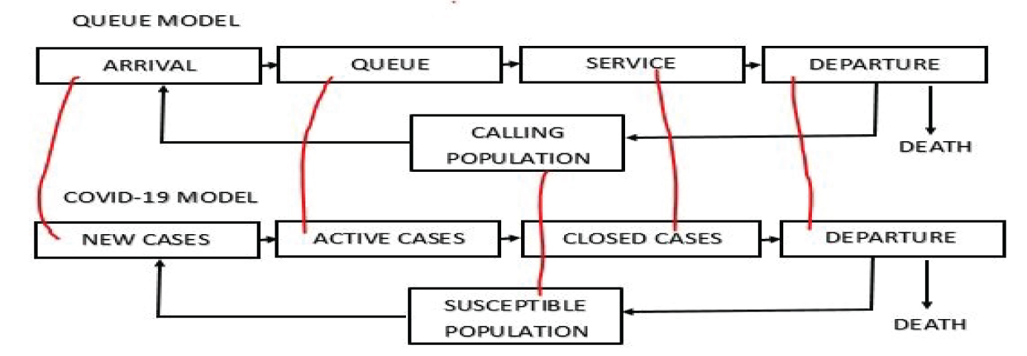 Figure 1: COVID-19 model as a Queue Model (http://creativecommons.org/licenses/by-nc-sa/4.0/).
View Figure 1
Figure 1: COVID-19 model as a Queue Model (http://creativecommons.org/licenses/by-nc-sa/4.0/).
View Figure 1
Thus, closed cases is given by
Closed cases = Recovered cases + Death
The active cases are those cases that are still on queue waiting for outcome (recovery or death).
Active cases = Total cases - Closed cases
The assumption of the COVID-19 model follows a simple queuing system. By the Kendall notation, we have
where the first M denotes the new cases (arrivals) and follows a Poisson distribution, the second M denotes the service times and follows a negative exponential distribution. The 1 denotes a single server, which implies that we are considering only one disease (COVID-19). The FCFS is the service discipline, it is assumed that first to be infected with COVID-19 is first to get an outcome (recovery or death). The first ∞ signifies the queue capacity, that is, the possible number of individuals that can be infected with the virus, and it is assumed to be infinite. The second ∞ signifies that the susceptible population is infinite. It is also assumed that there is no simultaneous arrival, that is, no two individuals can be infected at the same time. It is also assume that a COVID-19 infected individual remains infected until the individual is either recovers ordies.
The following mathematical notations are used in this study in relation with the models developed (Table 1).
Table 1: Mathematical notations. View Table 1
The probability of n infected individuals in a country at time t + δt are determined by summing up probabilities of all the possible ways this event could occur. The probability of occurrence of each of the event is given thus (Table 2).
Table 2: Possible states. View Table 2
P(event1) = Pn(t) × (1 - λdt) × (1 - µdt) (9)
P(event1) = Pn(t)[1 - λdt - µdt + λµ(dt)2]
P(event2) = Pn+1(t) × (1 - λdt) × (µdt) (10)
P(event2) = Pn+1(t)[µdt - λµ(dt)2]
P(event3) = Pn-1(t) × λdt(1 - µdt) (11)
P(event3) = Pn-1(t)[λdt - λµ(dt)2]
P(event4) = Pn(t) × λdt × µdt (12)
P(event4) = Pn(t)λµ(dt)2
Events 1 to 4 are mutually exclusive and exhaustive events. The probability Pn(t + dt) can be derived by adding the individual probabilities of event 1 to 4.
Pn(t + dt) = Pn(t)[1 - λdt - µdt + λµ(dt)2] + Pn+1(t)[µdt - λµ(dt)2] + Pn - 1(t)[λdt - λµ(dt)2] + Pn(t)λµ(dt)2 (13)
Pn(t + dt) = Pn(t) - λPn(t)dt - µPn(t)dt + µPn + 1(t)dt - λµPn + 1(t)(dt)2 + λPn - 1(t)dt - λµPn - 1(t)(dt)2, n > 0 (14)
where equation (14) is probability of having n cumulative cases in a country at time t + dt. It is necessary to solve for Pn(t + dt) when n = 0. In this case, only two mutually exclusive and exhaustive events can occur as shown in Table 3.
Table 3: Possible states. View Table 3
P(event1) = P0(t) × (1 - λdt) × 1
P(event1) = P0(t)(1 - λdt) (15)
P(event2) = P1(t) × (1 - λdtµdt)
P(event2) = P1(t)[µdt - λµ(dt)2] (16)
Thus, Pn(t + dt) = P0(t)(1 - λdt) + P1(t)[µdt - λµ(dt)2] (17)
Pn(t + dt) = P0(t) - λP0(t)dt + µP1(t)dt - λµP1(t)(dt)2, n = 0. (18)
From equation (14)
Pn(t + dt) - Pn(t) = -λPn(t)dt - µPn(t)dt + µPn + 1(t)dt - λµPn + 1(t)(dt)2 + λPn - 1(t)dt - λµPn - 1(t)(dt)2 (19)
Dividing through by dt and taking the limit as dt → 0 gives
Similarly, from equation (18)
Dividing through by dt and taking the limit as dt → 0 gives
Equations (20) and (22) provide relationship involving the probability density function
(pdf), that is, Pn(t)∀n. Assuming the steady state system, the differential equations (20) and (22) reduce to difference equations (23) and (24) respectively.
Equations (23) and (24) can be solved simultaneously. From equation (3.16), we have
Setting n = 1 in equation (23) gives
0 = -λP1 - µP1 + µP2 + λP0 (27)
Also, setting n = 2 in equation (23) gives
0 = -λP2 - µP2 + µP3 + λP1 (29)
More so, setting n = 3 in equation (23) gives
0 = -λP3 - µP3 + µP4 + λP2 (31)
Now, setting n = k in equation (23) gives
0 = -λPk - µPk + µPk + 1 + λPk - 1 (33)
This pattern continues for all values of n > 0. Following the values of n = 1,2,3,...,k, we can conclude from the knowledge of mathematical induction that
The probability that there is at least an active COVID-19 laboratory confirmed case in a country is given by
The probability that there is no active case of COVID-19 individual in a country is P0. Thus,
ρ + P0 = 1,
so that
Thus, the probability that there will be n active case of individuals with COVID-19 in a country is given by
Traffic intensity:
Recall that
Taking the likelihood gives
Taking the log of the likelihood gives
Differentiating equation (40) with respect to λ gives
Equating equation (41) to zero and solving for λ gives
The traffic intensity is approximated by
This shows that the system is steady since < 1.
Similarly, differentiating equation (40) with respect to µ gives
Equating equation (44) to zero and solving for µ gives.
The traffic intensity is approximated by
This also shows that the system is steady since < 1.
The average number of COVID-19 infected individuals in a country of interest is estimated.
By definition
where k is the variable of infected individuals and Pk is the probability of infection.
Ls = (1 - ρ)[1 + ρ + 2 ρ2 + 3 ρ3 + ⋯] (48)
Thus, the average number of active cases in a country per time is given by
Expected duration of COVID-19 infection in human is given by
Expected duration per COVID-19 individual to wait from infection recovery in a country,Wq is given by
The data used for this study is a time dependent data collected on COVID-19 new cases, total cases, new death, total death, new recovery, total recovery for four selected SSA countries: Nigeria, Kenya, South Africa and Central African Republic (CAR) from the time the first case of COVID-19 was confirmed in the country to 10th November, 2021. The data were compiled from four different sources, Worldometer, World Health Organisation (WHO), John Hopkins University database and Centre for Disease Control (CDC) of the respective countries. The four countries are selected using simple random sampling and quota sampling method. The simple random sampling method is used to obtain the four countries whereby each country has equal chance of being selected and then investigate a trait or a characteristic of each subgroup. One country each is selected from West, East, South and Central African countries.
The Table 4 shows the summary of the data as of 10th November 2021 for Nigeria, Kenya, South Africa and Central African Republic (CAR). It shows that South Africa, followed by Kenya, Nigeria has the highest number of COVID-19 confirmed laboratory cases among the selected SSA countries and also have the highest new cases (arrival), while Central African Republic has the lowest cases and did not record any new case as of 10th November 2021. The number of deaths and recovered cases are also in that order, South Africa, Kenya, Nigeria and CAR.
Table 4: Selected SSA countries COVID-19 data generated on 10th November 2021. View Table 4
The Figure 2 shows the active cases of COVID-19 in Nigeria, Kenya, South Africa and CAR as 5297, 1,254, 16426 and 4620 respectively. Kenya, despite having higher number of COVID-19 reported cases when compared with Nigeria and CAR, it has the least number of COVID-19 active cases among the selected SSA countries, accounting for only 5% among the selected SSA countries.
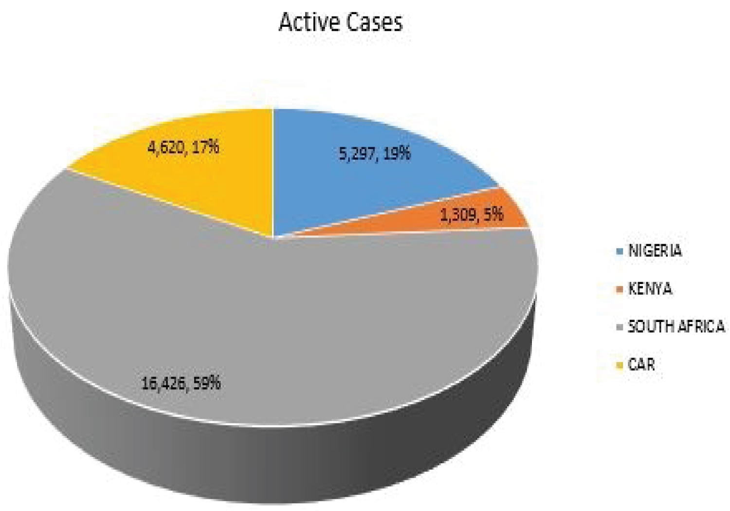 Figure 2: COVID-19 active cases of selected SSA countries.
View Figure 2
Figure 2: COVID-19 active cases of selected SSA countries.
View Figure 2
The Figure 3 shows the closed cases of COVID-19 in Nigeria, Kenya, South African and CAR as 207,597, 252,842, 2,908,196 and 6,959 respectively. South Africa accounts for 86% of the total closed cases and 59% of the total active cases among the selected SSA countries.
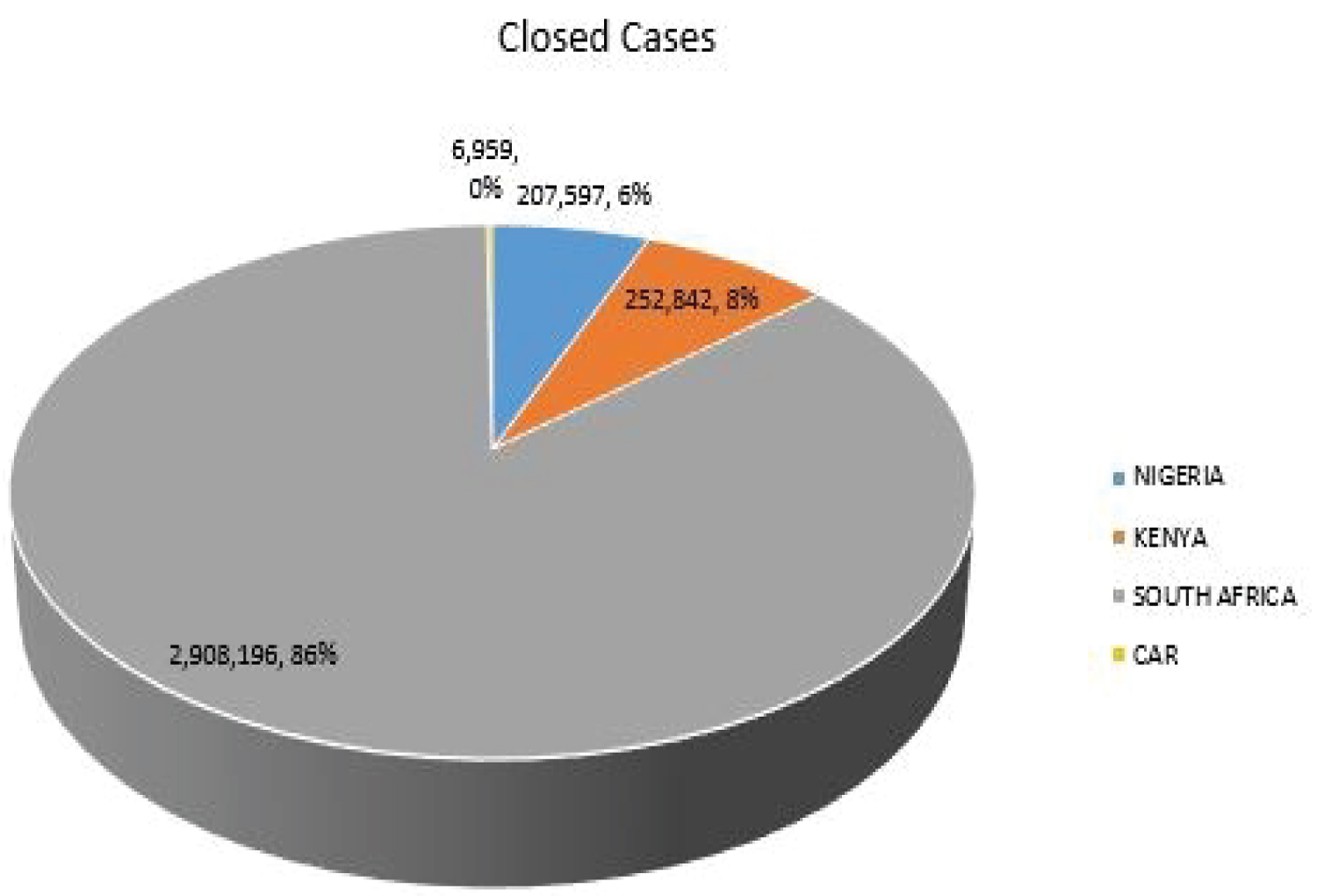 Figure 3: COVID-19 closed cases of selected SSA countries.
View Figure 3
Figure 3: COVID-19 closed cases of selected SSA countries.
View Figure 3
The Table 5 shows the MLE parameters of the model. The expected new cases per day (average arrival rate) of COVID-19 for Nigeria, Kenya South Africa and CAR are 375, 466, 5355 and4 respectively. The closed cases (cases with outcome) of COVID-19 in Nigeria, Kenya, South Africa and CAR are 384, 468, 5386 and 13 respectively. Since, the closed cases are more than the new cases, it implies that in the nearest future, the queue will be empty, meaning there will not be COVID-19 cases again. The probability that there is at least an active COVID-19 laboratory confirmed case in for Nigeria, Kenya South Africa and CAR are 0.97448, 0.99482, 0.99435, and 0.33611 respectively. The expected number of active cases per day in Nigeria, Kenya, South Africa and CAR are 37.2, 191.2, 175.1 and 0.2 respectively. It means that on the average daily cases of COVID-19 in Nigeria should be 37.2 cases per day, but as of 10th November 2021, the new confirmed cases are 65. The difference might be due to the average, which took account of days when there were high incidence and low incidence of COVID-19 cases, which affected the expected value. For Kenya, the MLE says 191.2 per day, while as of 10th November 2021 it was 178 for that days. For South Africa, the MLE is 175.1 as against 305 for the day under review; while for CAR the MLE is 0.2 as against 0 for the day under review.
Table 5: Maximum likelihood estimates of the model parameters. View Table 5
The Figure 4, Figure 5, Figure 6 and Figure 7 show that as time increased, the number of COVID-19 active cases in Nigeria, Kenya and South Africa decreased, while that of Central African Republic increased. Thus, the MLE parameters actually predicted the real life situation showing that COVID-19 cases with outcome are greater than new cases, thereby reducing the number of active cases per day.
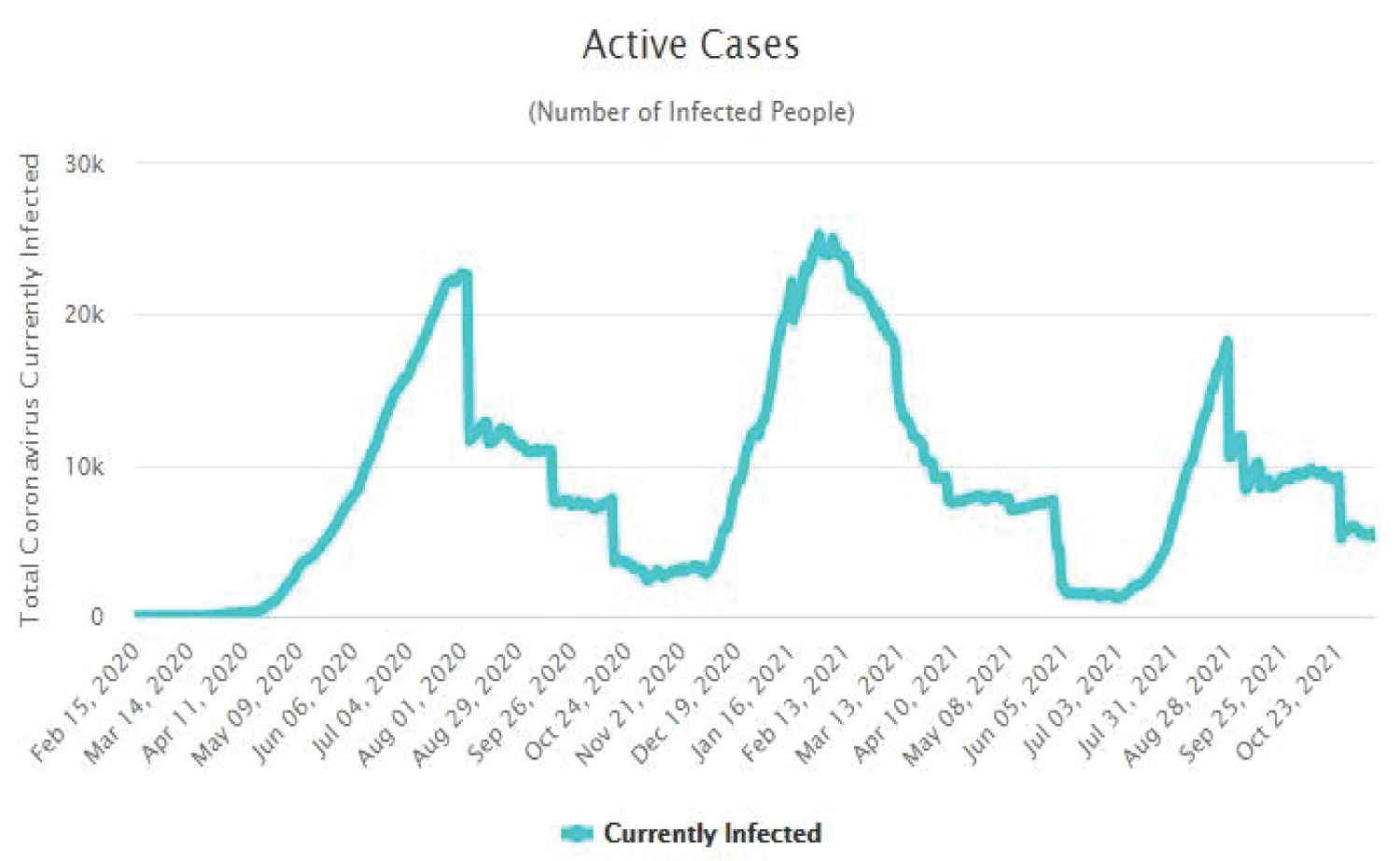 Figure 4: Time plot of COVID-19 active cases for Nigeria.
View Figure 4
Figure 4: Time plot of COVID-19 active cases for Nigeria.
View Figure 4
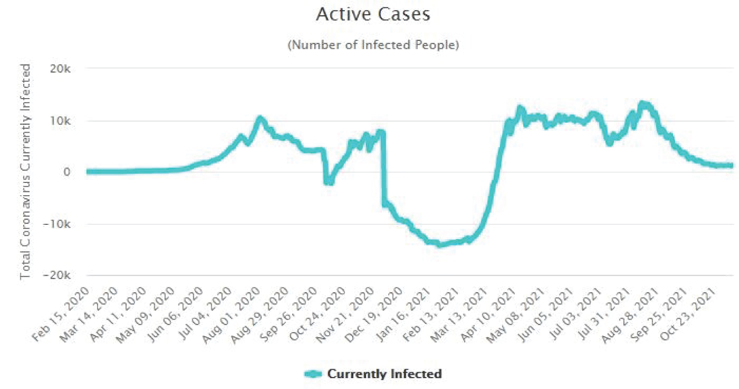 Figure 5: Time plot of COVID-19 active cases for Kenya.
View Figure 5
Figure 5: Time plot of COVID-19 active cases for Kenya.
View Figure 5
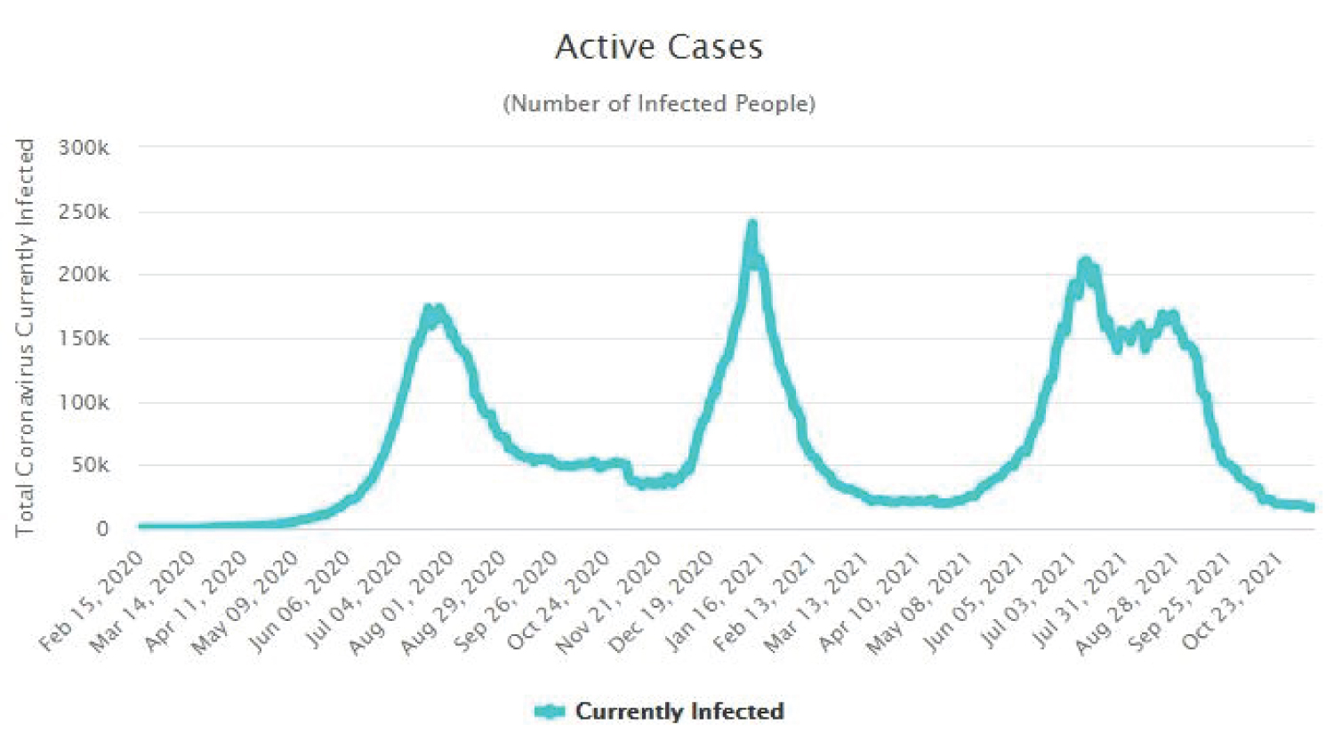 Figure 6: Time plot of COVID-19 active cases for South Africa.
View Figure 6
Figure 6: Time plot of COVID-19 active cases for South Africa.
View Figure 6
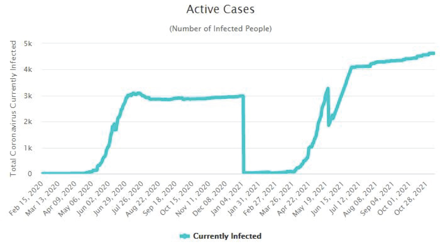 Figure 7: Time plot of COVID-19 for CAR.
View Figure 7
Figure 7: Time plot of COVID-19 for CAR.
View Figure 7
Figure 8 shows that the probability of recovery from COVID-19 is higher than its mortality rate. This implies that there is hope at the end of the tunnel for SSA countries. People that died of COVID-19 are not much when compared with people that recovered from the disease.
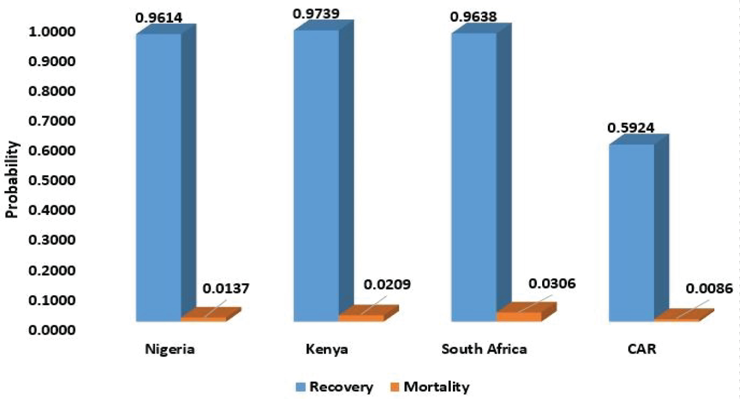 Figure 8: Probability of recovery and mortality of COVID-19.
View Figure 8
Figure 8: Probability of recovery and mortality of COVID-19.
View Figure 8
The research aimed to fit birth-and-death models using maximum likelihood estimation method with application to COVID-19 in Sub-Sahara African countries.
The probability distributions of infected, recovery and death of COVID-19 patient are determined using their respective steady state probabilities. The probability of recovery is above 0.9 for Nigeria, Kenya and South Africa, only Central African Republic has a low recovery rate, which is 0.5924, that is, 59.24% but also has a very low COVID-19 induced mortality rate of 0.0086 (0.86%). The highest mortality rate among the selected countries in SSA is South Africa with a mortality rate as low as 3.06%. This implies that the COVID-19 induced mortality rate for SSA countries is very low.
The steady state probability of getting infected with COVID-19 was derived using maximum likelihood estimation method. The estimated probability of infection for the selected countries shows that Kenya has the highest probability of getting infected with COVID-19, followed by South Africa, Nigeria, while the least is Central Africa Republic. It should however be noted that the average values for the period under study was used rather than the current value, this might affect the estimates. Nevertheless, the estimates show the real situation in the countries.
The probability of having more than a certain number of infected individuals in a susceptible population was derived using maximum likelihood estimation method. This can be termed as the probability of having more than n active cases in a population, where n is a natural number. Among the selected countries, Kenya has the highest probability of having more than 10 COVID-19 cases, followed by South Africa, Nigeria and Central African Republic in that order. The probability that there will be active cases in a population is higher for Kenya compared to other selected countries.
The study also estimated the average waiting time between infection and recovery/death of COVID-19 individual using maximum likelihood estimation. This is the average survival time of the virus in the body of an African. Among the selected countries, Kenya has the highest survival time for the virus, followed by Nigeria then Central African Republic. South Africa has the least survival time for COVID-19 virus in the system. This shows that Kenya as a slower time for an outcome of COVID-19 infected individuals.
The average number of COVID-19 infected individuals per day was derived. Kenya has the highest number of COVID-19 active cases per day, followed by South Africa then Nigeria. Central African Republic has the least average number of COVID-19 active cases per day. The number of active cases per day is dependent on the total number of new cases and closed cases. If the number of closed cases is higher than the number of new cases, then the system is at a stable state, and with time the active cases will reduce to zero, provided the reverse is not the case.
The authors declare that they have no known competing interests.
No financial assistance was received for this study.