In Argentina, Aedes aegypti represents an important public health threat, since it is the vector responsible for the transmission of dengue, chikungunya, zika and yellow fever. Mundo Sano Foundation has been carrying out periodic surveys of immature vector stages in several cities of northern Argentina. The main tool to mitigate their spread is through vector control. The identification of vector "hot spots" is an important key to design preventive program tools. Geostatistical techniques such as spatial autocorrelation (SAC) and kriging interpolation can be used to predict vector abundance in unsampled areas using data obtained from monitored sites. The knowledge of the spatial autocorrelation of vector abundance is fundamental and it can also be used to design disease surveillance strategies: To determine the characteristics of chemical control; to select ovitrap placement (distance between samples); and to determine the optimum sample size, among others. It is important to analyze the effect of the variation of the scale in the observed phenomenon.
This paper analyzes a two years series of weekly oviposition data from 25 ovitraps distributed in the urban area of a small city (104 measurements were collected for each ovitrap). We aim to understand how the relationship between sites measurements varies considering its relative location in the city, for different temporal sampling frequency or temporal resolution (TR). Different similarity measures between curves and graphic representations of these relationships, are explored. Among these, an innovative use of polar graphs -a tool commonly used to detect changes in satellite images- is examined. We evaluate variograms and SAC for multitemporal data (oviposition curves) at each TR.
Similarity between curves does not show spatial continuity in relation to the spatial arrangement of ovitraps, may be due to the effect of processes that are only observable at the microhabitat scale or due to sociodemographic factors. As the temporal resolution is greater in a given area, a greater number of ovitraps are needed to capture the spatial heterogeneity of the abundance of the vector. At the maximum TR analyzed, the minimum distance of spatial correlations was set at 1000 m. This has implications on the quantity of ovitraps per area unit required in the field in order to obtain a good description of the population dynamics of Ae. aegypti at the peridomestic level.
The results would indicate that when varying the time scale of analysis, the spatial scale should be modified accordingly to adapt to the new data structure. The ability to predict ecological phenomena depends on the relationships between spatial and temporal scales. The approach and innovative statistical tools described in this study, based on empirical data from a field study, may be used by different Ae. aegypti monitoring and control programs in order to design and implement tailor-made interventions. It would allows to support not only the selection of field samples, and to obtain data interpolation parameters, but also to contribute to the development of vector abundance models.
Spatio-temporal scales, Aedes aegypti, Oviposition, Distance curves
Aedes aegypti is of great sanitary importance in Latin America, since it is the main vector for dengue, chikungunya, zika and yellow fever viruses. Dengue is one of the most widespread vector-borne diseases in the world [1] and continues increasing in annual incidence as well as in geographical expansion [2]. Particularly, in Argentina, Ae. aegypti is the most relevant mosquito from an epidemiological point of view. Its main characteristics are its domiciliary habitat in urban areas [3], its breeding preference for artificial water containers rather than natural water bodies, and the resistance of its eggs to desiccation [4].
There is a lack of effective vaccines for most of the viruses, the main tool to mitigate their spread is through vector control. Traditional control measures include: a) The elimination of larval habitats, using chemical treatment, to prevent adult production and b) The application of spatial aerosol insecticides to reduce adult population density [5]. Despite of the resistance vector and environmental concerns, chemical control still remains the main strategy of vector control programs; however the World Health Organization (WHO) and the Pan-American Health Organization (PAHO) jointly promote its combination with other non-chemical vector control strategies [6]. For this reason, the identification of vector "hot spots" is an important key to design preventive program tools [7].
An increase in vector density would lead to an increase in human-vector contacts, which would result in a higher rate of viral transmission among the population [8]. Thus, the detection of changes in vector abundance is an important factor in the epidemiology of the disease [9]. There are several widely used entomological indexes to determine vector abundance, among them: 1) Indexes related to the presence or absence of the vector (larval indexes such as Housing and Breteau index); 2) Estimation of absolute abundance (method of tagging, release and recapture, aspiration of mosquitoes inside and outside houses, sampling of pupae), and 3) Estimation of relative abundance (ovitraps, females attracted by human bait, traps for adult mosquitoes). Ovitraps are a standard tool for monitoring the presence of Ae. Aegypti and its spatial activity [10]. This tool consists in offering a breeding site for Ae. aegypti to lay its eggs and it is basically a container with water. Some of the advantages of ovitraps as a method to evaluate the relative abundance of Ae. aegypti (number of eggs per ovitrap) are their low cost; the possibility to place them outside the houses, avoiding having to enter the household; and their easy maintenance. An important application of the data obtained are double; on the one side, it allows for the evaluation of control activities through the reduction in the mosquito population and on the other, it allows for the calculation of the mosquito density threshold required for arbovirus transmission. The number of eggs found in the ovitraps, together with the Housing and Breteau indexes (number of positive recipients found in the households related to the amount of the total inspected ones), provide a profile of vector abundance. Through continuous recording of mosquito oviposition, it is possible to study the spatial dynamics of vector populations [11], to calculate the annual infestation rate and to establish periods with high levels of gonadotrophic activity.
Through spatial analysis of entomological and epidemiological variables it is possible to address the challenges of dengue surveillance, and define more effective intervention strategies [12]. In particular, geostatistical techniques such as spatial autocorrelation (SAC) and kriging interpolation can be used to predict vector abundance in unsampled areas using data obtained from monitored sites [13]. The knowledge of the spatial autocorrelation of vector abundance is fundamental and it can also be used to design disease surveillance strategies: To determine the characteristics of chemical control [14]; to select ovitrap placement (distance between samples); and to determine the optimum sample size, among others. For example, the distance between the sampling sites might be adequate for a given mosquito species, but not for another one due to differences in dispersion and/or distribution of the two species [15]. Some studies have evaluated the spatial autocorrelation of abundance data from an ovitraps site [15,16], deriving recommendations regarding the design of dengue surveillance programs. However, there is a lack of published studies that analyze the spatial autocorrelation of multitemporal data of ovitraps (oviposition curves).
On the other hand, scale plays a central role in determining the outcome of observations [17]. As working scales change, statistical relationships may change, including the magnitude or sign of correlations, important variables, and variance relationships. Then, it is important to analyze the effect of the variation of the scale in the observed phenomenon.
Within this context, Mundo Sano Foundation (MSF), a non-profit organization, has been carrying out a Monitoring and Control Program of Ae. aegypti in several cities of northern Argentina which includes the periodic survey of immature stages of the vector by seasonal outbreaks of dengue. This program includes Ae. aegypti monitoring with ovitraps as a routine activity. MSF is located in strategic areas of Argentina, where neglected diseases such as chagas, soil-transmitted helminths, dengue, leishmaniasis and echinococcosis are present. Their work is conducted by local teams in collaboration with the local authorities and the communities affected. Their aim is to create models that can serve as proof-of-concept so that they may be are replicatedble and escalatedble, so by others they are implemented in different scenarios and taking into consideration the singularities of the communities involved.
Through this study, we attempt to understand how the relationship between ovitrap measurements at each site varies as a function of their relative position in an urban locality and the time series of the analysis. Therefore, the specific objectives proposed are:
• To define a measure of distance, or similarity between oviposition data temporal series, in order to be able to capture the most important components of the variability between these curves;
• To analyze the distance between Ae. aegypti egg abundance curves (i.e. time series of ovitraps samplings) with respect to their spatial location and to the sampling temporal resolution;
• To evaluate the behavior of the respective variograms and the spatial dependence (or autocorrelation) for each sampling frequency.
In order to achieve this, different measurements of distance between oviposition time series and graphic representations of these relationships were explored. Among these, the innovative use of polar graphics stands out, a tool commonly used to detect changes in satellite images. The tools used in this study prove to be useful for the design and implementation of monitoring and control programs of Ae. aegypti.
This work contributes in both, the methodological and the epidemiological point of view since the understanding of interactions between spatial and temporal scales of the problem will help decision makers to planning control actions. The results would be useful in control programs to identify priority areas and to allocate resources more effectively.
In this study, data resulting from the field work performed by MSF in localities in the North of Argentina are analyzed. In particular, a two year series of weekly data from 25 ovitraps distributed in the urban area of Clorinda, a small city in northern Argentina, is used.
The city of Clorinda (25° 17JS, 57° 43JW ), which is the second city in importance of the province of Formosa, Argentina, is the head of the Pilcomayo department, and is located on the right bank of the Pilcomayo River approximately 10 km from the mouth in the Paraguay River (Figure 1). According to the last national census in Argentina, from 2010, the city has 16,600 homes and its population is 23,290 [18]. It belongs to the humid Chaco region and represents a subtropical climate with no dry season. The average annual temperature is around 23 ℃ and the average annual precipitation is about 1300 mm, due to a rainy season extending from October to May [19].
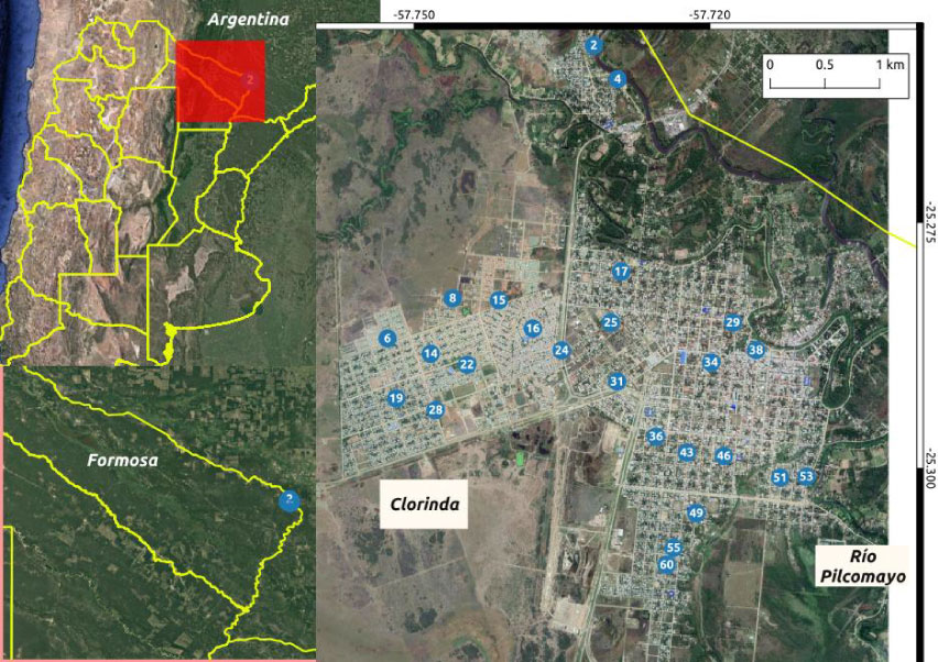 Figure 1: Study area located in the city of Clorinda, head of the Pilcomayo department. The positions of the 25 outdoor ovitraps are indicated.
View Figure 1
Figure 1: Study area located in the city of Clorinda, head of the Pilcomayo department. The positions of the 25 outdoor ovitraps are indicated.
View Figure 1
In Clorinda, MSF carries out surveillance and control actions in a total of 63 homes. From these, a subset of 25 houses was selected based on the simultaneous and continuous number of measurements obtained over the entire study period of the current study (Figure 1). Ovitraps were used to measure weekly oviposition in the selected houses. Ovitraps consisted of black cylindrical plastic containers that were 12 cm high with a 10 cm diameter. The traps were filled around half way with water and wood tongue depressors (15 × 2 cm) were placed inside each one. The tongue depressor acts as a substrate for the eggs so that they can be posteriorly counted. Tongue depressors were replaced in a weekly manner. For each household, two ovitraps were used, one in the inside and the other one in the peridomicile, preferably in a shaded area out of the reach of children and pets. The oviposition database includes the number of positive households, number of positive ovitraps, and the number of eggs for each epidemiological week. The traps are checked every 6 days (giving to vector enough time to lay its eggs). This paper analyzes the external ovitrap data corresponding to a two-year time period from August 2014 (epidemiological week 31 of 2014) to July 2016 (epidemiological week 30 of 2016). Therefore, 104 measurements were collected for each ovitrap over the two years.
All calculations required by the methodology described bellow were carried out using the R statistical software [20]. The pseudocode of the routines is presented in Appendix 1A.
Various statistical measures of distance (dissimilarity or difference) were used in order to determine the variation between the egg abundance curves obtained from each individual ovitrap. Herein, we describe two of the evaluated distance measures explored:
Given two vectors, t and r, that store the time series of egg abundance obtained by ovitraps at two given sites, B components or dimensions (b = 1,...,B), it is possible to define two types of distances:
• Magnitude, defined as the Euclidean distance:
Where tb and rb are the bth components of vectors t and r. It measures the degree of change, the amplitude of the temporal curve of oviposition values. The variable magnitude carries information about the presence/absence of changes.
• Direction, defined as the cosine of the angular distance:
Where tb and rb are the bth components of vectors t and r. Therefore, as a way to evaluate the distance between curves, the concept of Spectral Angle Mapper (SAM), i.e. an algorithm widely used in Change Detection Analysis in remote sensing, was followed. According to this, the spectral similarity between two samples can be obtained by considering each spectrum as a vector of q dimensions, where q is the number of bands, in our case it is the number of dates. SAM determines the spectral similarity by calculating the angle between two spectra by treating them as vectors in a space with dimensionality equal to the number of bands [21]. It is related to the type of change reflected in the periodicity, seasonality, or the frequency of the curve of temporal distribution of oviposition values.
These distance measurements can be represented in polar coordinates (magnitude and direction variables respectively) in a polar graph as presented in section 4.7.1.
In our case study, each oviposition curve (corresponding to a single ovitrap site) was compared to the average time evolution of oviposition of all households taken as a reference. The reference curve is displayed in Figure 2.
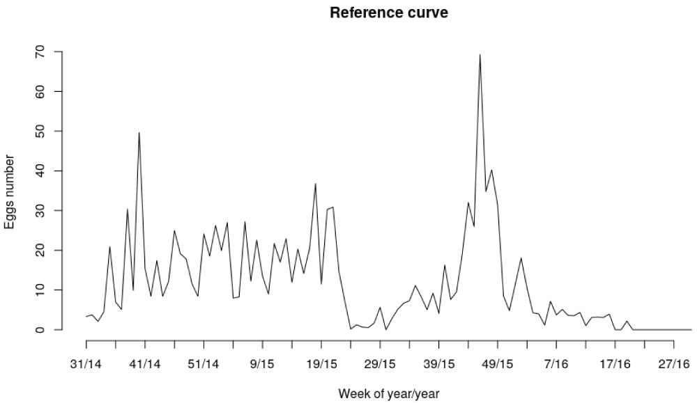 Figure 2: Average time evolution of oviposition of the households taken as a reference curve. The horizontal axis represents the time axis, a/b where a indicates the epidemiological week and b indicates the year. The vertical axis is the average number of eggs found in the 25 ovitraps.
View Figure 2
Figure 2: Average time evolution of oviposition of the households taken as a reference curve. The horizontal axis represents the time axis, a/b where a indicates the epidemiological week and b indicates the year. The vertical axis is the average number of eggs found in the 25 ovitraps.
View Figure 2
Different temporal resolutions (TR) of sampling were defined by resampling the data. The original series of data from the 104 oviposition measures obtained from the outdoor ovitraps from each household were resampled through down sampling or decreasing the frequency of samples, using a statistical average operator. Then the TR coding is Xw meaning that for the resampling 1 data was taken every X weeks. For instance, 2w means that 1 data was taken every 2 weeks.
The variogram is a statistic that is used to quantify the spatial correlation between sampled values. It is calculated as the average squared difference between two points separated by given a distance |h|. The variogram indicates how different or dissimilar the values between two sites are. Because the values of a regionalized variable are not independent, an observed value in a given site provides information about the values of neighboring sites. The range in a variogram is the maximum distance at which one point influences another one. Measurements separated by a distance less than the range are spatially correlated. This concept of range may imply consequences on the selection of samples. Whereas the sill is the value at which the model first flattens out.
For each considered TR, the fitness of variograms for the variable ρt,r, i.e. distance ρ between curves t and r, where r is the reference curve; was performed using the gstat package of R statistical [22]. Then, the trend of the resulting ranges with respect to the decrease in the sampling frequency (decrease in TR) was analyzed and a Linear regression model was adjusted for TR and the range variables.
We report Multiple R2 (Coefficient of Determination) and Adjusted R2 in order to provide a measure of the proportion of total variation of outcomes explained by the model.
• Multiple R2 (Coefficient of Determination) represents the percent of the variance of Y intact after subtracting the error of the model:
The bigger the error, the worse the remaining variance will appear.
• Adjusted R2 normalizes Multiple R2 by taking into account how many samples you have and how many variables we are using:
Polar charts are a useful tool to display information in polar coordinates. The polar coordinate system is a two-dimensional coordinate system in which each point of the plane is determined by a radius ρt,r and an angle αt,r. The values of magnitude are represented by the distance from the points to the center of the circle, the farther the point is from the center; the greater is its magnitude.
The direction or cosine angular distance, is related to how temporarily close the curves are (seasonal dynamics), while the magnitude (Euclidean distance) is related to the difference in egg quantity.
In addition to polar charts, we explored the potential use of a graphing method that uses a matrix of correlation between variables as input. In particular, the qgraph package for R [23] provides an interface to visualize data through network modeling techniques. For instance, a correlation matrix can be represented as a network in which each variable is a node and each correlation an edge; by varying the width of the edges according to the magnitude of the correlation, the structure of the correlation matrix can be visualized. In our case, this matrix is not a correlation but a table in which the columns and rows correspond to the different ovitraps and the value of the cell for each row and column is the value of the distance (magnitude or direction) between these curves.
Figure 3 and Figure 4 display the curves that have greater distance between them with respect to magnitude and to direction, respectively. This example shows the oviposition curves at maximum TR. The reference curve is shown to facilitate the visualization of the relationships. The magnitude reflects the abundance difference between curves while the direction highlights the temporal phase shift between them.
 Figure 3: Curves with maximum difference in magnitude (curves of ovitraps e16 and e36). The reference curve (Rc) is also shown.
View Figure 3
Figure 3: Curves with maximum difference in magnitude (curves of ovitraps e16 and e36). The reference curve (Rc) is also shown.
View Figure 3
 Figure 4: Curves with maximum difference in direction (curves of ovitraps e15 and e4). The reference curve (Rc) is also shown.
View Figure 4
Figure 4: Curves with maximum difference in direction (curves of ovitraps e15 and e4). The reference curve (Rc) is also shown.
View Figure 4
Figure 5 shows the results of the synthesis processing performed on the reference curve at four different temporal sampling resolutions: 3, 6, 9 and 12 weeks.
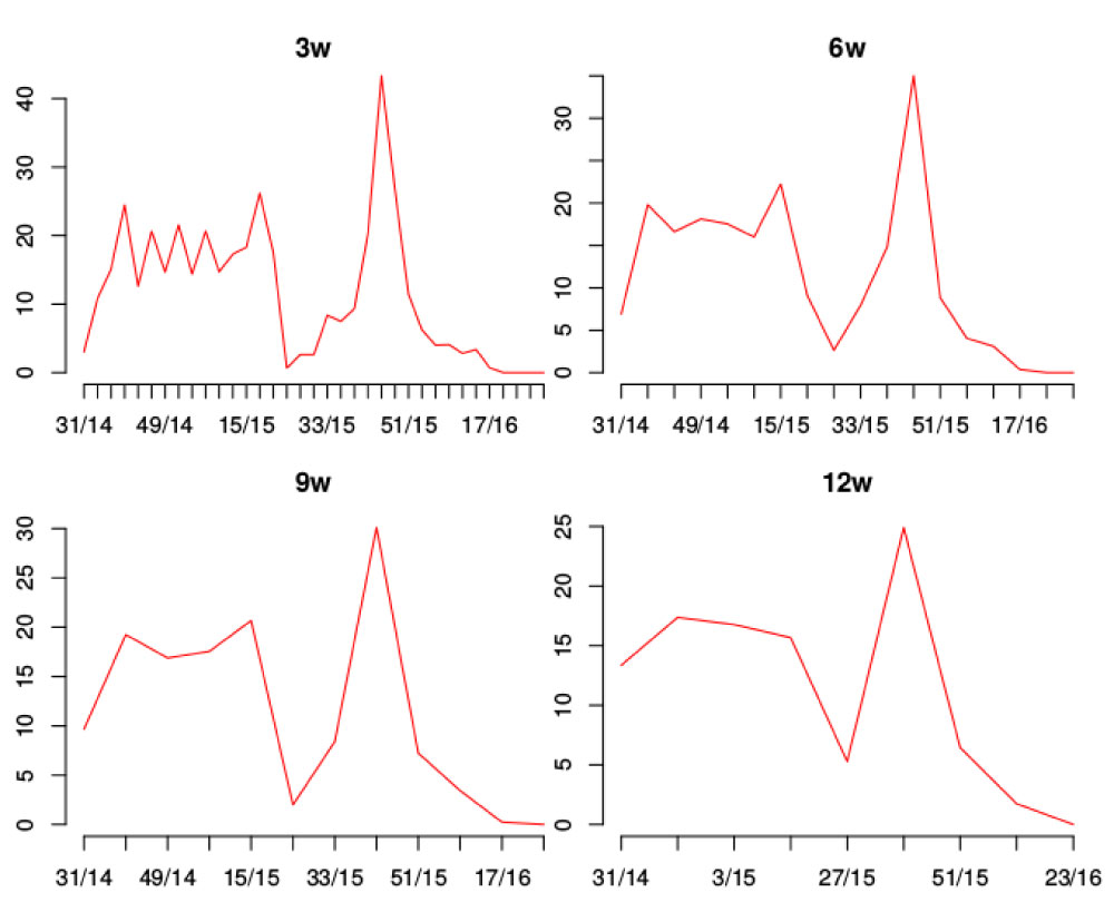 Figure 5: Reference curve according to the different temporary resolutions: 3w, 6w, 9w, 12w. Horizontal axis shows week of year/year marks. Vertical axis shows egg number.
View Figure 5
Figure 5: Reference curve according to the different temporary resolutions: 3w, 6w, 9w, 12w. Horizontal axis shows week of year/year marks. Vertical axis shows egg number.
View Figure 5
Table 1 list the parameters of the variograms adjusted to the variable ρt,r, for each TR. A spherical model was adjusted using the gstat package of R [22]. In Figure 6 and Figure 7 the variogram of the minimum and maximum TR, respectively, are shown.
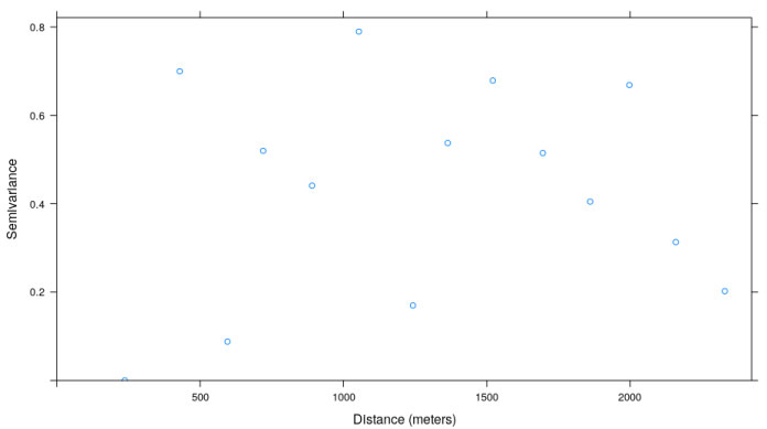 Figure 6: Variogram ρt,r (distance ρ between curves t and r, with r being the reference curve). B = 1, only the week 32/14 is considered.
View Figure 6
Figure 6: Variogram ρt,r (distance ρ between curves t and r, with r being the reference curve). B = 1, only the week 32/14 is considered.
View Figure 6
 Figure 7: Variogram ρt,r (distance ρ between curves t and r, with r being the reference curve). B = 104, 104 weeks are considered, that is, the maximum TR.
View Figure 7
Figure 7: Variogram ρt,r (distance ρ between curves t and r, with r being the reference curve). B = 104, 104 weeks are considered, that is, the maximum TR.
View Figure 7
Table 1: Variogram parameters adjusted via a spherical model. View Table 1
At the maximum TR analyzed (Table 1 and Figure 7), 1w, field sample sites should be separated from each other by at least 1000 m in order to ensure that two samples taken in the field are not statistically correlated.
It is observed that, as the TR decreases (the sampling frequency decreases), the distance between curves does not present spatial correlation as the spatial distance increases. Therefore, in order to obtain uncorrelated information, sites should be placed at greater spatial distances, from 1000 m for high temporal to almost 2000 m for low temporal resolution. These results have implications with respect to the number of ovitraps required per area unit in the field in order to obtain a good description of what is happening with Ae. aegypti in the peridomiciles.
At a minimum TR (only one week of the two years is sampled) the spatial regionalized structure is eliminated as shown in the variogram of Figure 6. The information structure for the spherical model is vanished. Therefore, complete spatial randomness is presented and, consequently, it is not possible to generate an interpolated map at a TR of less than 2 weeks.
When varying the time scale of analysis, the spatial scale should be modified accordingly to adapt it to the new data structure. A spatial pattern that was analyzed every 1000 m at a certain resolution or time scale may not be relevant at another time scale. At lower TR, the required distance of no correlation between ovitraps increases.
From Table 1, a linear regression model between the variables TR and range was fitted giving an adjusted R2 of 0.82. The TR variable was determinant for the correlation distance range, through a negative coefficient. That is, as the sampling frequency increases (TR increases), the range or decorrelation distance decreases, as shown in Figure 8 (Table 2).
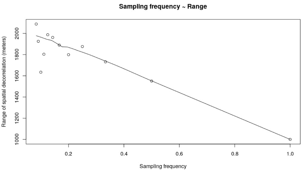 Figure 8: Parameter range of variograms adjusted following a spherical model with respect to temporal resolution (TR) or sampling frequency.
View Figure 8
Figure 8: Parameter range of variograms adjusted following a spherical model with respect to temporal resolution (TR) or sampling frequency.
View Figure 8
Table 2: Linear regression model parameters for range vs. sampling frequency (1/TR). View Table 2
Figure 9 is the graphical representation of the distance between the curves t and r (ρt,r and αt,r). Each ovitrap, t, is analyzed with respect to the reference curve, r, located at the polar graph origin. It is possible to observe that the curves more different in terms of magnitude, i.e, egg number, are 16 and 36 (Figure 3). For angular distance, the curves most distant from each other in terms of direction are ovitraps 4 and 15 (Figure 4).
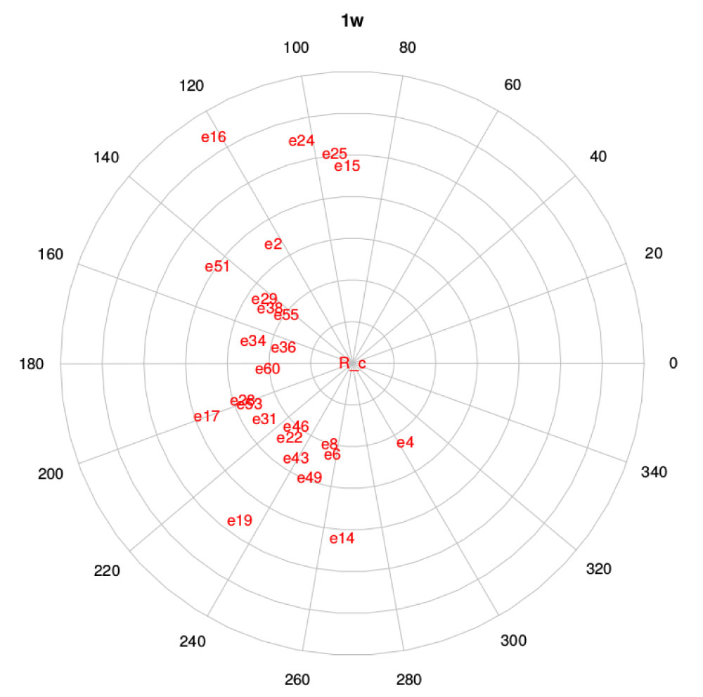 Figure 9: Polar graph corresponding to the polar coordinates (ρRc,r and αRc,r ) of distance between curves. e stands for external because it corresponds to the curves of the outdoor ovitraps and the number refers to the site number (r).
View Figure 9
Figure 9: Polar graph corresponding to the polar coordinates (ρRc,r and αRc,r ) of distance between curves. e stands for external because it corresponds to the curves of the outdoor ovitraps and the number refers to the site number (r).
View Figure 9
Again, it is possible to confirm that the spatial distance does not determine the distance between egg abundance curves.
In Figure 10, the network of relationships between curves is visualized considering the real spatial location between ovitraps and the Euclidean similarity is shown through the width of the link between nodes. Note that it is a plane representation in which each node is on the real location of the corresponding ovitrap.
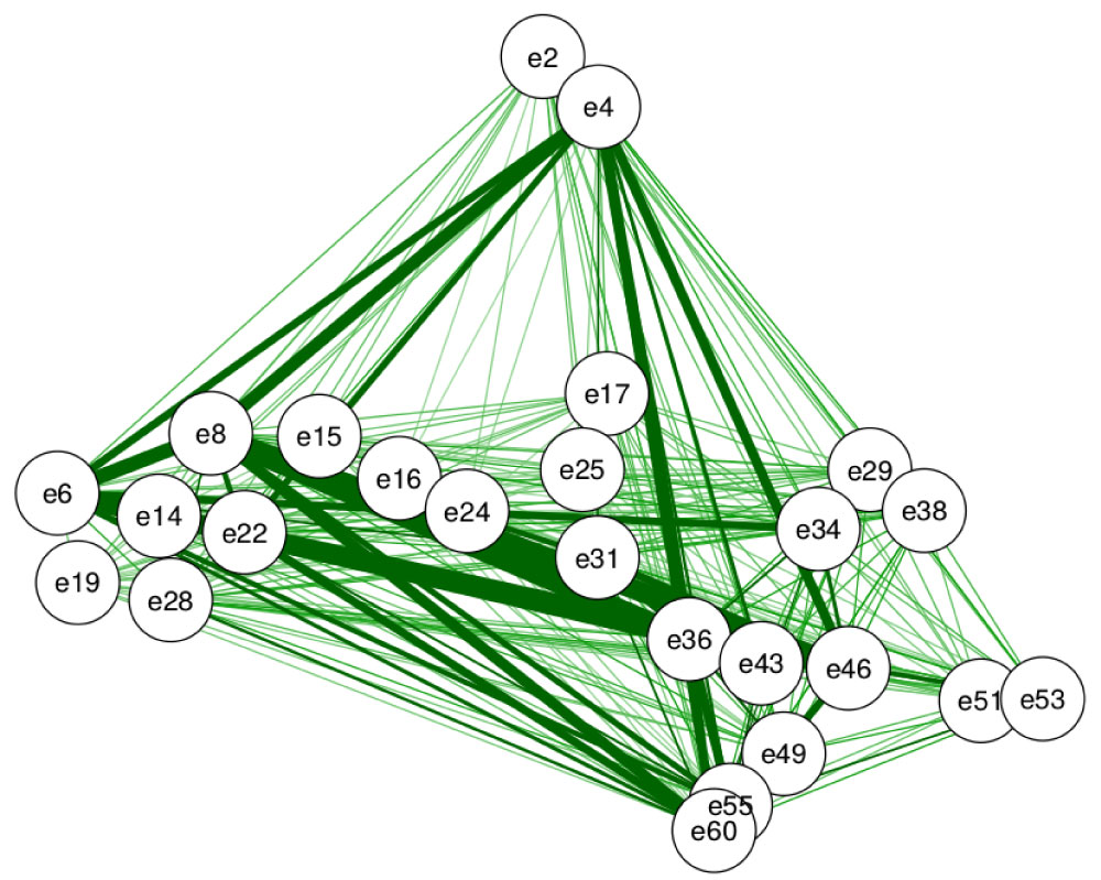 Figure 10: Weighted network visualization of the relationship between curve distances.
View Figure 10
Figure 10: Weighted network visualization of the relationship between curve distances.
View Figure 10
Studies conducted at different regions of Argentina showed different seasonal patterns. In general, oviposition activity is associated with variations in temperature and/or precipitation, but peak oviposition was recorded in different months in different Argentinian provinces [4]. A study conducted in Salta Province showed that oviposition activity of Ae. aegypti occurs throughout the year, with a peak in March (summer), which was related to an increase in precipitation [24]. In the case of Chaco Province, the maximum number of eggs and immature abundances were found in November-December (spring), in Córdoba in December-January (summer) and in Buenos Aires in February-March (summer). These differences are probably the consequence of rainfall and temperature dynamics across the latitudinal gradient. In the current study from the province of Formosa, and according to the average reference curve, the peak of abundance of eggs would be recorded in October or November (spring) coinciding with Chaco (neighboring province). Recent studies like Heinisch, et al. [25] confirm that seasonal variation of the oviposition rate of Ae. aegypti would be mediated by the maximum and minimum temperatures.
The measures of similarity or distance defined here allow us to analyze not only the magnitude of change between time series but also the type of change with respect to the frequency of the curve. Polar graphs, as presented in this paper, represent an innovative tool to visualize differences between series of temporal data (Figure 2). In this study, the effect of varying the reference curve in the distance analysis was not evaluated. This could be a limitation since the use of different reference curves (or an average reference curve) could result in different distance patterns. In relation to the analysis at different temporal resolutions of sampling, as expected, the characteristics of oviposition become more similar (grouped in terms of both, magnitude and angle) as we lose temporal detail.
The distance of each oviposition curve to the reference curve is not related to spatial or geographical distance (Figure 1, Figure 9 and Figure 10). Beyond the time scale at which the polar graph corresponding to the ratio of distances between curves is observed, it seems that the pattern of similarity between curves does not show spatial continuity in relation to the spatial arrangement of ovitraps. There are factors beyond the local environmental determining the oviposition curves. It is therefore interesting to analyze which factors (environmental, micro-environmental, socioeconomic, and demographic, among others) determine the spatial pattern of recorded oviposition curves.
Several studies performed in Argentina have evaluated how environmental factors influence oviposition dynamics. Some of these factors include gradient and type of urbanization [18,26-28], percentage of exposed soil [27], distribution and type of water bodies [18,27], density of vegetation [18] and presence of water containers [28], among others. In Clorinda, the high-density breeding areas of Ae. aegypti are characterized by a deficit in the supply of drinking water, especially during the summer months [29], promoting the accumulation of a large variety of water storage containers near homes.
The lack of spatial continuity in the similarity between curves may be due to the effect of processes that are only observable at the microhabitat scale or due to sociodemographic factors. Therefore, further studies need to be conducted in order to understand intra-city dynamics and their micro-regulation. On the one hand, there is evidence that at the microhabitat scale, the presence of immature stages increases in locations that are less exposed to sunlight, with higher and more closed vegetation and with a shaded and vegetated environment [30]. On the other hand, Almirón, et al. [31] did not find differences in the number of eggs from ovitraps located in sites that were under different sunlight exposure conditions. Another study noted that critical oviposition areas observed in heat maps seemed to coincide with places of high poverty, pointing to the influence of socio-demographic factors [32].
With respect to the spatial correlation measured through the variograms, different sampling time resolutions resulted in different decorrelation distances. Somehow the range defines the distance of separation between the ovitrap sites. If the temporal frequency of sampling is decreased, the spatial samples should be further apart in order to keep statistical independence (Table 1). In other words, when the temporal resolution is greater in a given area, a greater number of ovitraps are needed to capture the spatial heterogeneity of the abundance of the vector. This has implications on the quantity of ovitraps per area unit required in the field in order to obtain a good description of the population dynamics of Ae. aegypti at the peridomestic level. Therefore, this would indicate that when varying the time scale of analysis, the spatial scale should be modified accordingly to adapt to the new data structure. This reinforces the concept that our ability to predict ecological phenomena depends on the relationships between spatial and temporal scales.
According to Albrieu-Llinas, et al. [18], the distance of spatial correlation could be determined by migration patterns of the vector, by environmental factors, or socioeconomic variables, since they are anthropophilic vectors. According to the literature, flight dispersion of Ae. aegypti is generally from 50 to 200 m [33] but other studies have reported distances of up to 400 m and 3.5 km [15,34-36]. Therefore, for the current study, the minimum distance of spatial correlations was set at 1000 m.
Distance measures between oviposition curves, their graphic representation, and the spatial correlation analysis of the aforementioned similarity measures, at different time scales, define an approach that can be applied to different urban and rural settings.
The approach and innovative statistical tools described in this study, based on empirical data from a field study, may be used by different Ae. aegypti monitoring and control programs in order to design and implement tailor-made interventions. In this way, it would allows to support not only the selection of field samples, and to obtain data interpolation parameters, but also to contribute to the development of vector abundance models such as those presented in Scavuzzo, et al. [37], Lana, et al. [38]. For instance, interpolation technique has been employed to estimate the occurrence of eggs of Ae. aegypti [25], to associate the vector distribution with the transmission of the pathogens [39], to identify the clustering of the malaria vectors [40] and to relate entomological indicators to the incidence of dengue [41]. In the same way, an example of how the operational generation of vector distribution and abundance maps can be used to define the strategy of insecticide application during an epidemiological outbreak can be found in Rotela, et al. [42] and Janet, et al. [43].