Our goal in this paper is to adapt to the context of the Greater Abidjan Region (Côte d'Ivoire) an existing model reflecting the evolution of the COVID-19 epidemic in Wuhan (China). This model is a deterministic compartmental model which is translated by a system of ordinary differential equations. We are reinvesting this model to obtain the parameters of the epidemic in the great Abidjan. We study some mathematical aspects of this deterministic model.
Using data from the evolution of the COVID-19 epidemic in Abidjan, we obtain constants corresponding to the Greater Abidjan Region epidemic. We are performing numerical simulations using these constants to predict the behavior of the epidemic in the Greater Abidjan Region.
The initial model does not take into account certain disturbances and sudden shocks which could disturb its behavior. In the Greater Abidjan Region, some continuous or sudden events disrupt the behavior of the epidemic. To stick to the realities of the Greater Abidjan Region, we introduce a white noise and jumps that correspond to the different disturbances that can occur. We obtain a stochastic model of COIVD-19 with jumps. We prove that our new model with jumps has a positive global solution. In certain conditions, this solution oscillates in the set of the disease-free equilibrium of the deterministic model. We perform numerical simulations which corroborate our theoretical results.
COVID-19 epidemic model, Disease-free equilibrium, Jump perturbation
This study aims at analyzing the evolution of the COVID-19 epidemic in the great Abidjan over the period of public measures application. For this reasons, we have worked on data related only to that period. For the next step, we plan to make predictions to account the evolution of this epidemic.
In [1], Pierre Magal, et al. develop a mathematic model for COVID-19 epidemic in Wuhan (China) in which the population was composed of four compartments:
• S(t) is the number of susceptible individuals at time t i.e., people who are not infected yet but might become infectious individuals in the future,
• I(t) is the number of asymptomatic infectious individuals at time t i.e., people who have contracted the disease but have not yet developed it at time t,
• R(t) is the number of reported symptomatic infectious individuals i.e., symptomatic infectious with severe symptoms at time t,
• U(t) is the number of unreported symptomatic infectious individuals i.e., symptomatic infectious with mild symptoms at time.
The instant corresponds to December 31, 2020. The epidemic starts at instant .
At this time, they noted , , and . Times are expressed in days and for they obtained:
, , , and are real constants on [0;1]. is the transmission rate.
is the rate at which the asymptomatic infectious individuals become symptomatic. They assume is the average time during which asymptomatic infectious are asymptomatic.
f is the fraction of symptomatic infectious that become reported symptomatic infectious. So is the rate at which asymptomatic infectious become reported symptomatic infectious.
is obviously the fraction of symptomatic infectious that become unreported symptomatic infectious. So
is the rate at which asymptomatic infectious become unreported symptomatic infectious.
is the rate at which the symptomatic infectious individuals lose their symptoms by death or healing. They get
the average time symptomatic infectious have symptoms.
Pierre Magal, et al. calculated the parameters of their model from the Wuhan epidemic data before public confinement and isolation measures.
A nonlinear adjustment method allowed them to obtain an expression of the CR function giving the cumulative number of reported symptomatic infectious individual at time t. They obtain that
As , they deduce .
For experimental reasons, they assume that the average time during which asymptomatic infectious are asymptomatic and the average time symptomatic infectious have symptoms are around 7 days. They get . From their data, they assume that f is in the interval [0.8 ; 1]. They use the value afterwards.
From all these results, they calculated the values of all the parameters corresponding to the epidemic of COVID-19 in Wuhan, notably the transmission rate and the basic reproductive number . Theoretically, they computed . The data of Wuhan epidemic permit them to obtain and before the public measures.
With numerical simulations they show the evolution of the epidemic in Wuhan without public confinement and isolation measures. By varying the parameters of the model, they use simulations to predict the peak of the epidemic.
Since January 23, public confinement and isolation measures have been taken in Wuhan. Pierre Magal, et al. considered the effectiveness of its measurements after January 25. They therefore modified their model with the following non constant transmission rate:
With these public measures, numerical simulations show that the epidemic in Wuhan will be eradicated. We quote them: "As a consequence of our study, we note that public health measures, such as isolation, quarantine, and public closings, greatly reduce the final size of this epidemic, and make the turning point much earlier than without these measures."
In our work, we use the first deterministic model of Pierre Magal, et al. (1.1) because we consider that it could reflect the dynamics of the epidemic in the Greater Abidjan Region as we will see later with the data of this region. We rephrase some starting notations. We study the system from an instant which we will define later. At this instant we note the state of the system. is the total population size before the epidemic. In this model, there is no birth or recruitment. So, we have .
In section 1, we prove that the solution of the system (1.1) is bounded in .
Obviously is the set of the different disease-free equilibrium for the system (1.2). By using the LaSalle's global invariance principle [2,3], we show that all the solutions of (1.3), bounded for in , converge in M when . These mathematical results comfort us in the possibility of reaching a state without the disease.
In Côte d'Ivoire, the Greater Abidjan Region includes the city of Abidjan and six other districts which are peripheral.
In Côte d'Ivoire, the first patient of COVID-19 was detected in Abidjan on March 11, 2020. At the start of the epidemic, the rest of the country was unaffected by the disease. So the public authorities took the following measures [4].
• The suspension of air flights to countries with more than 100 reported cases (decided on March 20, 2020).
• The closure of all land, sea and air borders from midnight on March 22, 2020 until further notice.
• On March 23, 2020 the state of emergency is established. A curfew is in place from 9 p.m. to 5 a.m. for two weeks.
• From March 29, 2020, no transport is authorized between the Greater Abidjan region and the rest of the country.
• On April 9, 2020, it was decided: the wearing of the mandatory mask in the Greater Abidjan; compulsory confinement of fragile people; reduction of non-essential travels and the number of people in vehicles.
The Greater Abidjan Region is the epicenter of the epidemic with 98 percent of the confirmed cases. Since March 29 the big Abidjan has been isolated from the rest of the country. The rest of the country has no more than 5 reported cases. Since at least April 21, 2020, the rest of the country has no COVID-19 patients. National data in [4] can therefore be assimilated to that of the Big Abidjan (Table 1, Table 2, Table 3, Table 4, Table 5 and Table 6).
Table 1: Data of the COVID-19 epidemic in greater Abidjan Region from March 11 to March 20. View Table 1
Table 2: Data of the COVID-19 epidemic in greater Abidjan Region from March 21 to March 31. View Table 2
Table 3: Data of the COVID-19 epidemic in greater Abidjan Region from April 1 to April 10. View Table 3
Table 4: Data of the COVID-19 epidemic in greater Abidjan Region from April 11 to April 20. View Table 4
Table 5: Data of the COVID-19 epidemic in greater Abidjan Region from April 21 to April 29. View Table 5
Table 6: Data of the COVID-19 epidemic in greater Abidjan Region from April 30 to May 05. View Table 6
The majority of the economic activities of the Ivorian population are activities of the informal sector (small trade, rustic restaurant, street vendors, illegal taxi drivers,...). These activities mainly focus on the city of Abidjan. This did not allow the establishment of total containment in Côte d'Ivoire. In addition to conventional barrier measures (washing hands regularly, coughing in the elbow...), the measures above have been gradually implemented to curb the epidemic. As our study is limited to the Greater Abidjan Region, we will analyze the data from the isolation of the Greater Abidjan Region (March 30, 2020). We will therefore study our model with the eradication measures implemented.
On the other hand, from this isolation date, the epidemic data are more reliable because of the multiplication of screening centers.
These measures, which do not correspond to total containment, favor the transmission of the virus. The transmission rate of the Greater Abidjan Region model is therefore not zero.
In section 2, as was done in [1,5,6], we will determine the constants of the system (1.1) corresponding to the epidemic in the Great Abidjan Region with the effect of the public measures. We consider the period of the effect of the public measures for two reasons: daily statistical data is more significant during this period because of the multiplication of screening centers and we want to know the behavior of the epidemic with these measures. We use the software CurveExpert Pro to fit our data. That permits us to compute the different parameters of the Greater Abidjan Region model and the basic reproductive number . Simulation with MatLab software permits us to find the peak of the epidemic in the Greater Abidjan Region in the case of this deterministic model. Simulations with other parameter values make it possible to observe a more rapid eradication of the epidemic and to propose measures to achieve this.
In Côte d'Ivoire, continuously, certain protective measures such as minimum physical distance of one meter, regular hand washing etc. are not respected in markets and public transport vehicles. Abidjan has many large markets in each of its districts. Our region has many uncontrolled urban transport that does not allow compliance with health measures. Also, the practice of economic activities in the informal sector promotes many contacts between individuals. All these factors continually disturb the transmission rate of the model and could be assimilated to white noise to be introduced into the system (1.1). That's why we add a white noise to the model (1.1) to disrupt the transmission rate.
The isolation of the Greater Abidjan Region is not fully respected despite the efforts of the police. Sudden inflows or outflows of people take place formally with administrative authorizations or illegally by village roads.
Sudden mid-term measures such as the obligation to wear a mask and a curfew extension caused sudden shocks to the model at the first time when they were applied.
The model described by the system (1.1) does not take these factors into account. We need to introduce jumps in the system (1.1) to represent these sudden changes which disturb the transmission rate.
As in [7-9] and from the model (1.1) we develop a model with jumps perturbation that disrupt the disease transmission rate. We get the system. (1.2)
(1.2)
where is a Brownian motion defined on a stochastic basis and is constant.
-) means the left limit of , is a Poisson counting measure with the stationary compensator and is defined on a measurable subset Z of with .
In Section 3, we prove that the system (1.2) has a unique global and positive solution. We show how the jumps influence the behavior of the solution around the set of the equilibrium states. Inspired by [10,11] and using MaLab R2019b software, we perform numerical simulations which corroborate our theoretical results.
Here we justify simple mathematical properties that confer biological significance to our model.
N is the size of the population before the epidemic. We have . We prove that for any initial state in , the solution of the system (1.1) are bounded in .
For any given initial value in , the set is positively invariant for the system (1.1).
With the system (1.1), we obtain by summing the equation of the system:
If we prove that for , then will be decreasing and therefore less than or equal to that .
On the other hand, initiating the solution of system (1.1) in positive orthant , we have :
So the solutions of system (1.1) remain in at any time t, i.e. S, I, R and U are positive. We thus obtain the desired result.
Starting from any initial condition, the following result guarantees us, under certain conditions, the convergence of any solution in the set of the disease-free equilibrium for the system (1.1).
If , all the solutions of (1.1) bounded for in , converge in M the set of all the disease-free equilibrium for the system (1.1) when .
We define by .
Since all the model parameters are non-negative, and , we get :
So we have Since all the model parameters are non-negative and , we deduce that .
Moreover,
.
The only compact invariant subset of is . So, by Lasalle's global invariance principle, all the solutions (1.1), bounded for in , converge in M when .
In practical terms, when , any solution of the system (1.1) converges towards a disease-free state.
In this section, we will try to determine the parameters of the deterministic model corresponding to the dynamics of the epidemic in the Greater Abidjan Region after the implementation of all the public measures that led to its isolation.
As in [1] :
• , the average time during which asymptomatic infectious are asymptomatic is equal to 7 days and .
• , the average time during which symptomatic infectious have symptoms is equal to 7 days and .
All this brings us to consider our data 14 days after the isolation of the Greater Abidjan Region to tend towards the dynamics of the epidemic after all the public measures have been taken.
The initial instant of our study of the epidemic in the big Abidjan with the effect of public measures therefore corresponds to April 12, 2020. In our case we will name the state of the system at this time. This is the initial state of the model that we are going to study.
We will not use the value of indicated in [1] by Pierre Magal, et al. We will consider that . It is assumed in [12] and [13] that the young age of an individual favors the absence of symptoms or the development of very weak symptoms after COVID-19 contraction. The last population census of Côte d'Ivoire [14] shows that children (0-14 years-old) represent 41.8 percent of the total population and young people (15-34 years-old completed) constitute 35.5 percent of the total population. 77.3 percent of the total population is under 35 years of age. This extreme youth of the population could explain the low number of symptomatic infectious because the symptoms of the disease rarely appear. On the other hand, the low attendance of health facilities (around 47 percent, [15]) may not favor the detection of COVID-19. Screening is only systematic in the event of serious symptoms and symptomatic infectious are hardly detected. There are not enough screening centers, although their number has been increased. For all these reasons, we will assume that around 5 percent of infectious individuals become confirmed cases. and .
The parameters , , and therefore and are thus known.
is the size of the population of the big Abidjan before the epidemic.
We know the number of reported cases at t=0 (April 12, 2020) : .
As in [1], we define the CR function of the cumulative number of reported symptomatic infectious cases at time t for with the function
where is the solution of .
The statistical data of the COVID-19 epidemic show that the variations in the number of susceptible people due to the epidemic in the beginning of the epidemic are so small so we can consider and because as we will see later the distance between 0 and is small. That will permit us to evaluate the other parameters of the model. We can later adjust the value of .
As we look at the epidemic from the effect of the measures at date t = 0 then, for , exists but has no interesting biological significance and is used just for calculations (Figure 1).
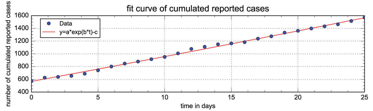 Figure 1: We display daily data for the cumulative number of cases reported from April 12, 2020 (t = 0). The fit curve equation is y = 11959.70832011228 × exp (0.003209387788757992 × t) - 11392.25601164384.
View Figure 1
Figure 1: We display daily data for the cumulative number of cases reported from April 12, 2020 (t = 0). The fit curve equation is y = 11959.70832011228 × exp (0.003209387788757992 × t) - 11392.25601164384.
View Figure 1
To exploit this adjustment function, we consider that For where the values of a, b and c are defined above.
When we use the methods to estimate the parameters presented and justified in [1] in section 4 we obtain that :
and
From the previous expressions and the determination of the previous parameters, we calculate the others constants of the model of the COVID-19 epidemic in the great Abidjan with the effect of public measures. We get , , , and .
With MatLab software, from the date of (April 12, 2020, ), the effect of all the public measures, we propose a simulation of the current situation in the Greater Abidjan Region with the constants previously determined. Let's recap.
The transmission rate is . The rate at which the asymptomatic infectious individuals become symptomatic is . is the fraction of asymptomatic infectious that become reported symptomatic infectious. So .
The rate at which asymptomatic infectious become unreported symptomatic infectious is
is the rate at which the symptomatic infectious individuals lose their symptoms by death or healing. The basic reproductive number for our deterministic model is .
At , , , , and . We get the following numerical simulations with MatLab sofware where we will not present the trajectory of the susceptible people because of a question of scale (Figure 2).
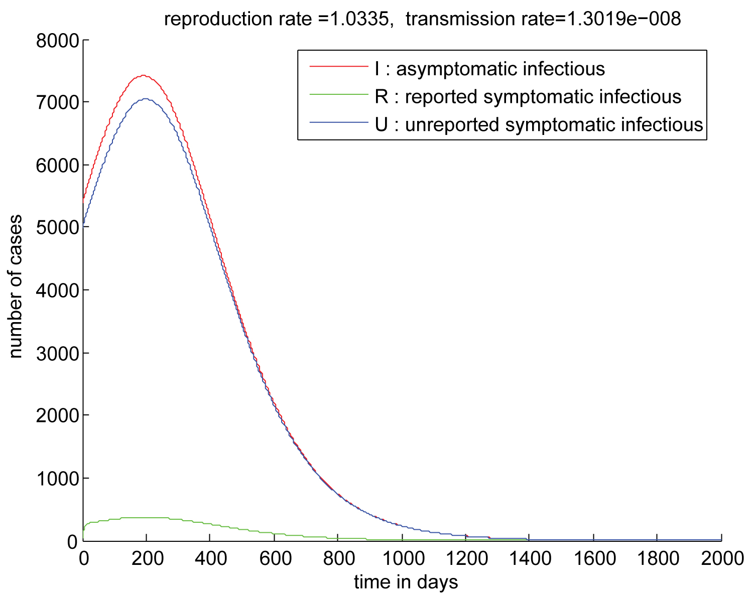 Figure 2: Trajectory of the solution without the suseptibles compartment of the deterministic system which describe the dynamic of the COVID-19 epidemic in the Greater Abidjan Region with the effect of the public measures. and . Peak of epidemic appears approximately 230 days after April 12, 2020.
View Figure 2
Figure 2: Trajectory of the solution without the suseptibles compartment of the deterministic system which describe the dynamic of the COVID-19 epidemic in the Greater Abidjan Region with the effect of the public measures. and . Peak of epidemic appears approximately 230 days after April 12, 2020.
View Figure 2
Now we present the evolution of susceptible individuals (Figure 3).
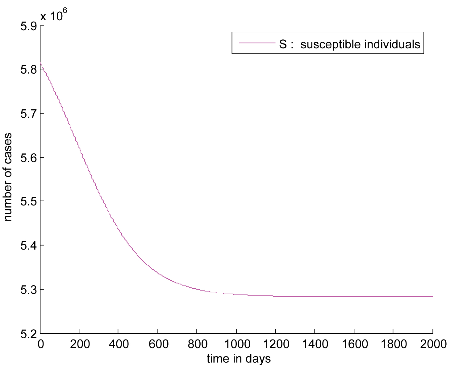 Figure 3: Trajectory of suseptibles compartment of the deteministic system which describe the dynamic of the of the COVID-19 epidemic in the Greater Abidjan Region with the effect of the public measures. and . Peak of epidemic appears approximately 230 days after April 12, 2020.
View Figure 3
Figure 3: Trajectory of suseptibles compartment of the deteministic system which describe the dynamic of the of the COVID-19 epidemic in the Greater Abidjan Region with the effect of the public measures. and . Peak of epidemic appears approximately 230 days after April 12, 2020.
View Figure 3
Under the conditions we have adopted, the epidemic in the Greater Abidjan lives around 1400 days after April 12, 2020, with a peak reaching 230 days after this date.
We can see that at the end of the epidemic, the number of susceptible people in the population of the big Abidjan is around 5,300,000. This drop should not be seen as deaths but rather as cures because the death rate from the disease is very weak (it is less than 1 percent as the statistics indicate. Refer also to the linear graphs). At the end of the epidemic, we have approximately 300,000 cured which does not influence the dynamics of the model.
In support of the public measures taken, we agree with the two new directions taken by the government of Côte d'Ivoire:
• Increase in screening tests,
• Repression and punishment of people who do not respect public measures and protective gestures.
An increase in screening tests results in an increase in the parameter and therefore in the rate .
We suggest a large increase from to 0.8. We hope that 80 percent of the infected will be reported cases in order to get them out of the dynamics of the epidemic.
The degree of repression and sanction can result in a coefficient k between 0 and 1 by which the current transmission rate is multiplied. If the repression and the sanctions are high then k is small and the rate of transmission decreases. For our simulation, we opt for k = 0.5, i.e. a reduction by half of the current transmission rate. With the previous values of the other parameters, using the same methods of parameter approximations the following simulation gives (Figure 4).
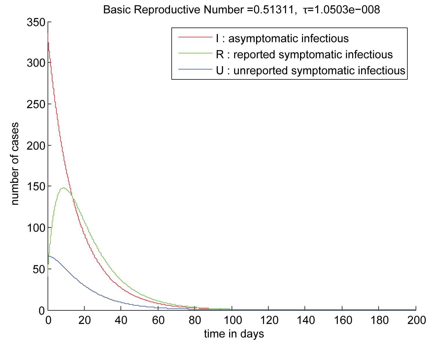 Figure 4: Trajectory of the solution without the suseptibles compartment of the deteministic system which describe the dynamic of the of the COVID-19 epidemic in the Greater Abidjan Region with the effect of the public measures. A vast screening campaign, sanctions and repression. For that we take A new transmission rate equal to where is the old transmission without repression. is coefficient that measures the intensity of sanction and repression. We takes and we obtain and . From the first moment the number of asymptomatic infections individuals is decreasing, the number of reported knows a peak after 15 days and the epidemic disappears 100 days after April 12, 2020.
View Figure 4
Figure 4: Trajectory of the solution without the suseptibles compartment of the deteministic system which describe the dynamic of the of the COVID-19 epidemic in the Greater Abidjan Region with the effect of the public measures. A vast screening campaign, sanctions and repression. For that we take A new transmission rate equal to where is the old transmission without repression. is coefficient that measures the intensity of sanction and repression. We takes and we obtain and . From the first moment the number of asymptomatic infections individuals is decreasing, the number of reported knows a peak after 15 days and the epidemic disappears 100 days after April 12, 2020.
View Figure 4
The following simulations shows in the same conditions the evolution of the number of individuals susceptible which knows a small decrease to stabilize at 5,815,600 at the end of the epidemic (Figure 5).
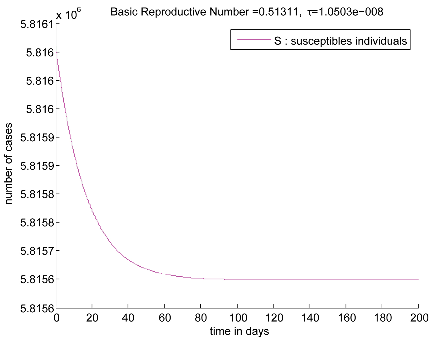 Figure 5: Trajectory of the suseptibles compartment of the deteministic system which describe the dynamic of the of the COVID-19 epidemic in the Great Abidjan with the effect of the public measures from April 12, 2020, a vast screening campaign, sanctions and repression. For that we take A new transmission rate equal to where is the old transmission without repression. is coefficient that measures the intensity of sanction and repression. We takes and we obtain and . From the first moment the number of asymptomatic infections individuals is decreasing, the number of reported knows a peak after 15 days and the epidemic disappears 100 days after April 12, 2020.
View Figure 5
Figure 5: Trajectory of the suseptibles compartment of the deteministic system which describe the dynamic of the of the COVID-19 epidemic in the Great Abidjan with the effect of the public measures from April 12, 2020, a vast screening campaign, sanctions and repression. For that we take A new transmission rate equal to where is the old transmission without repression. is coefficient that measures the intensity of sanction and repression. We takes and we obtain and . From the first moment the number of asymptomatic infections individuals is decreasing, the number of reported knows a peak after 15 days and the epidemic disappears 100 days after April 12, 2020.
View Figure 5
In this section, we study the model (1.2) for where represents the date of April 12, 2020, the date from which we assume that the public measures are effective.
Lyapunov analysis [7,8,16], permits us to prove that the solution of model (1.2) is positive and global.
We assume that the jump coefficient satisfies the following conditions:
\begin{itemize}
• where
with
• is a bounded function and there exists a strictly positive constant such that .
We will first prove that the system (1.2) has a unique solution which is global and positive. In a second point we will study the asymptotic behavior of this solution in the case . Simulations carried out with Matlab software confirm our results.
As in [16], we show that jump processes can suppress the explosion.
Theorem 6.1: With the assumptions and , for any given initial value , the equation (1.2) has a unique global solution for all
Proof: For any given initial value there is a unique local solution on a random interval where is the explosion time because of and the fact the drift and diffusion are locally Lipchitz.
To prove this local solution is global, we need to show that a.s. We will also prove that for any given initial value , the equation (1.2) has its solution
for all
At first we prove that the solution is positive. In second part, we prove that the solution checks for all
The set with or or or is not empty cause at , is in this set. So we define the following stopping time
Let be so large that
For , we define the stopping time
Clearly, is increasing as a.s. Set , whence, a.s.
If we can show that a.s is true, then a.s then the solution is global and positive a.s.
For , we define F a -function by .
Let and be arbitrary. For ,
is well defined.
Applying Itô's formula, we obtain
where
For , , live in $ [0;m]$ and is constant. As and live in [0;1], we get
We are in conditions where , and are dominated by positive constants. So, there is a strictly positive real constant such that
In other words by using the assumption , the fact , live in [0;m] for and the fact
is defined on a measurable subset with , we find a strictly positive real constant such that
Finally
Therefore,
Taking expectation, yields
We define for each 0,
Due to the property of the function $ F $ defined by , we see that
We know that if X is a Levy process then, for each we have almost surely where
S, R, I and $ R $ are Levy processes. So we obtain almost surely from (3.1) :
We deduce
Letting yields
Since T is arbitrary, we must have
a.s.
So a.s. and the equation (1.2) has a unique global positive solution for .
Now we prove that the solution is dominated.
Let be fixed in . is a deterministic function such that
is a positive constant. As we have shown above, and ) are positive for we can deduce that for , the deterministic function is a decreasing function.
Therefore for , .
The initial state being taken in
, therefore we have for
By varying in the universe of probability , we thus show that:
for ,
This completes our proof and for any given initial value
, the equation (1.2) has a unique global solution for all
Considering that , we prove that the solution of the stochastic system (1.2) oscillates in the set of the disease-free equilibrium for the deterministic system (1.1).
Theorem 6.2: Let , be the solution of the system (1.2) with initial value. If , then there exists such that
where .
Proof: We know that
Define a -function by
The function G is positive definite on , and
where
..
We obtain
Thereafter,
and
Since all the model parameters are non-negative, and , we get :
Since all the model parameters are non-negative and , we deduce that
Using that for , and the fact that the function C is dominated by a positive real , there is a real T such that
Hence,
Integrating both sides of (3.2) from 0 to t, then taking expectation, yields
By (3.3) we have
Therefore
Where
Remark 6.2: When the solution of (1.2) oscillates more closely in the set M of the disease-free equilibrium for the system (1.1) as the intensity of the noise and the jumps decrease. The case fatality rate is less than 1 percent (see linear graphs). Convergence towards a disease-free state is an encouraging sign. It is a disease-free situation with few deaths.
As in [7,10] using MatLab R2019b software, we add white noise and Poisson jumps to the first example seen in the deterministic case which reflects the reality in the big Abidjan. To be close to the difficulties of lowering the transmission rate in greater Abidjan, we lowered this rate by 10 percent in the first two figures and by 25 percent in the last two. We get basic reproductive numbers less than 1.
We obtain the following figures which corroborate the results of our last theorem (Figure 6).
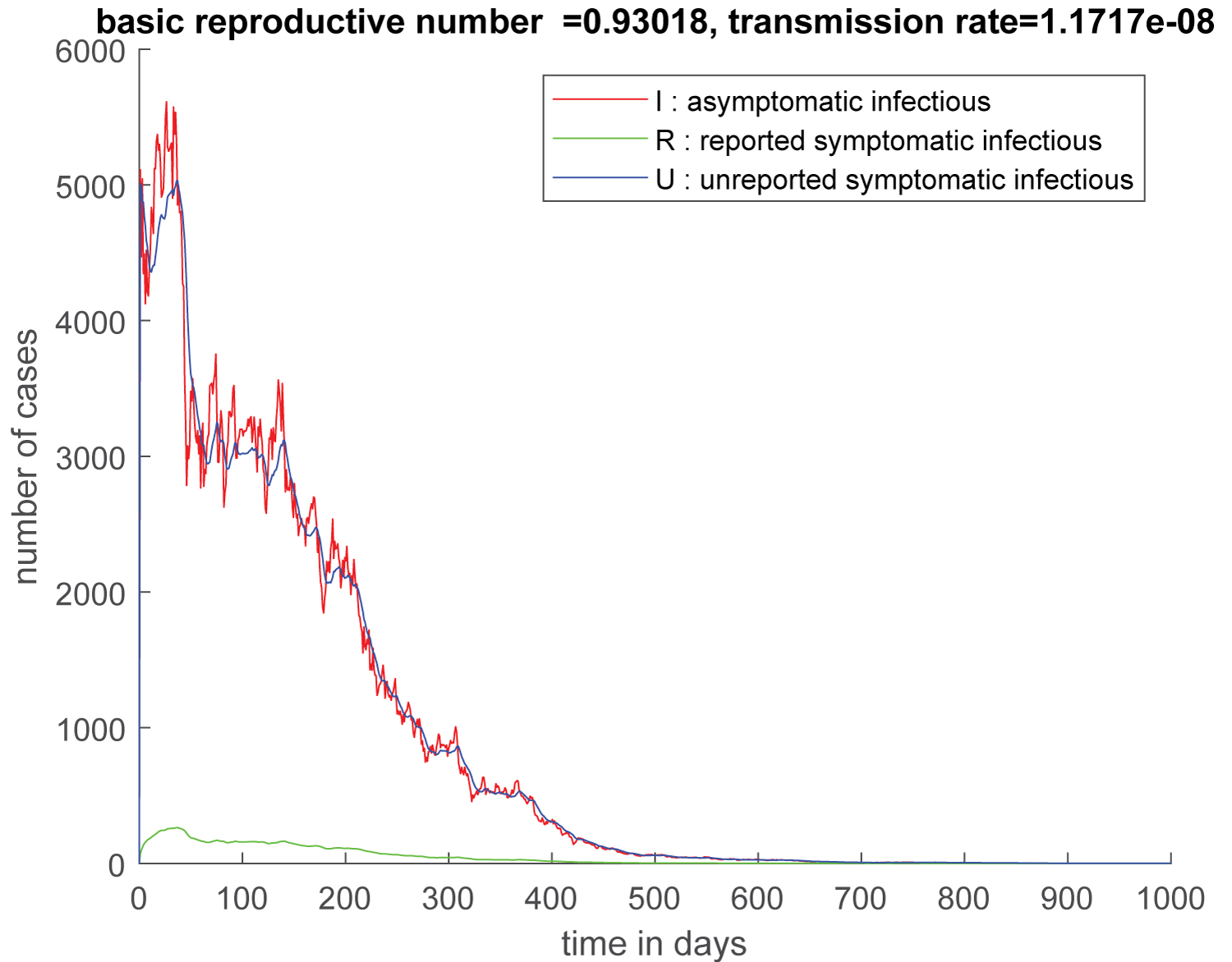 Figure 6: Trajectory of the solution without the suseptibles compartment of the stochastic system which describe the dynamic of the of the COVID-19 epidemic in the great Abidjan with the effect of the public measures from April 12, 2020. and Peak of epidemic appears to be around 600 days after April 12, 2020.
View Figure 6
Figure 6: Trajectory of the solution without the suseptibles compartment of the stochastic system which describe the dynamic of the of the COVID-19 epidemic in the great Abidjan with the effect of the public measures from April 12, 2020. and Peak of epidemic appears to be around 600 days after April 12, 2020.
View Figure 6
Now we present the evolution of susceptible individuals (Figure 7 and Figure 8).
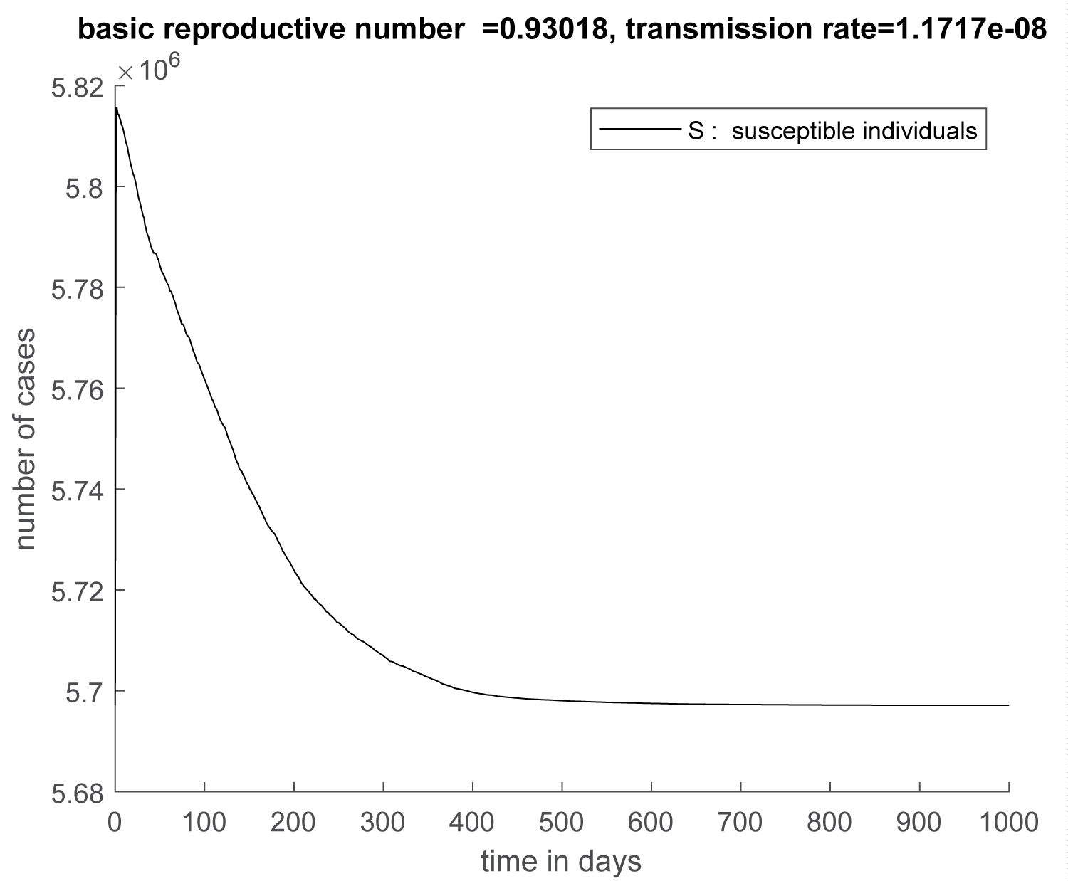 Figure 7: Trajectory of suseptibles compartment of the stochastic system which describe the dynamic of the of the COVID-19 epidemic in the great Abidjan with the effect of the public measures from April 12, 2020. and Peak of epidemic appears to be around 600 days after April 12, 2020.
View Figure 7
Figure 7: Trajectory of suseptibles compartment of the stochastic system which describe the dynamic of the of the COVID-19 epidemic in the great Abidjan with the effect of the public measures from April 12, 2020. and Peak of epidemic appears to be around 600 days after April 12, 2020.
View Figure 7
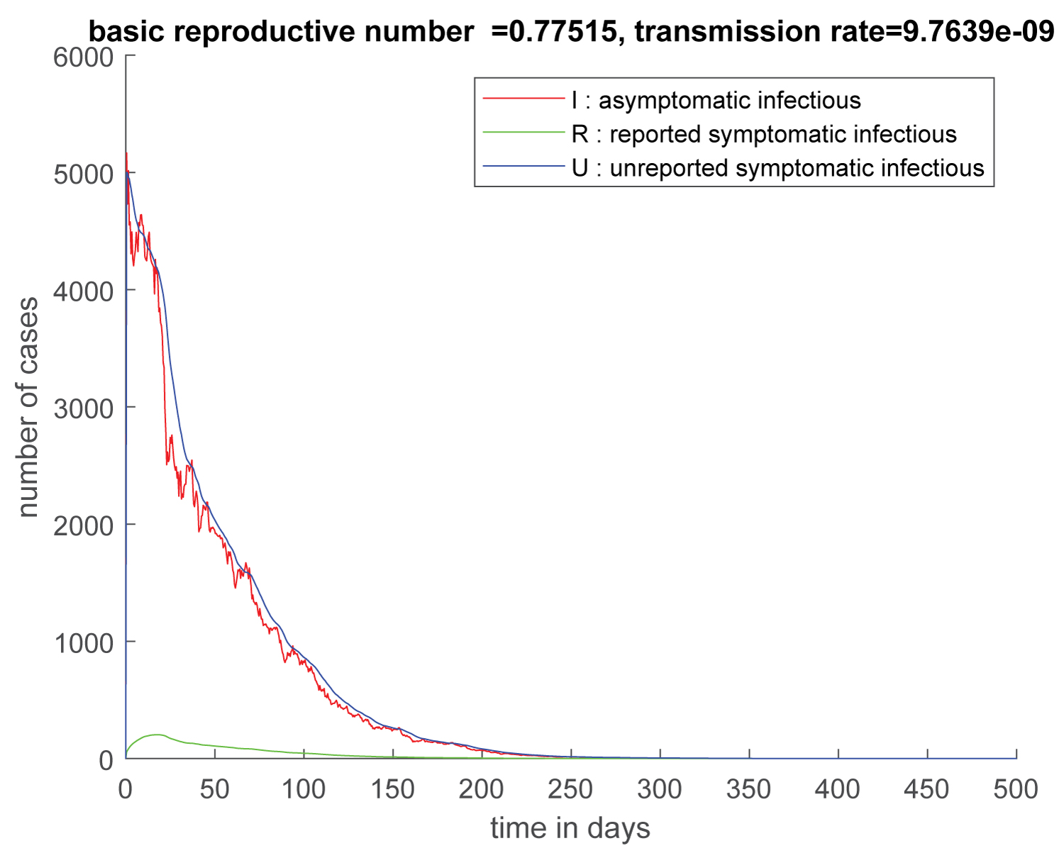 Figure 8: Trajectory of the solution without the suseptibles compartment of the stochastic system describe the dynamic of the of the COVID-19 epidemic in the Greater Abidjan Region with the effect of the public measures. and Peak of epidemic appears approximately 250 days after April 12, 2020.
View Figure 8
Figure 8: Trajectory of the solution without the suseptibles compartment of the stochastic system describe the dynamic of the of the COVID-19 epidemic in the Greater Abidjan Region with the effect of the public measures. and Peak of epidemic appears approximately 250 days after April 12, 2020.
View Figure 8
Now we present the evolution of susceptible individuals (Figure 9).
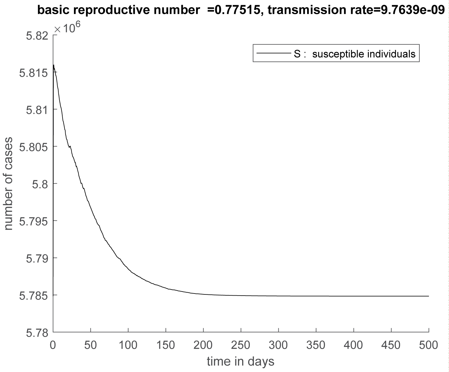 Figure 9: Trajectory of suseptibles compartment of the stochastic system describe the dynamic of the of the COVID-19 epidemic in the Greater Abidjan Region with the effect of the public measures from April, 2020. and Peak of epidemic appears approximately 250 days after April 12, 2020.
View Figure 9
Figure 9: Trajectory of suseptibles compartment of the stochastic system describe the dynamic of the of the COVID-19 epidemic in the Greater Abidjan Region with the effect of the public measures from April, 2020. and Peak of epidemic appears approximately 250 days after April 12, 2020.
View Figure 9
In this study, we tried to describe the behavior of the COVID-19 epidemic in the great Abidjan during the period of public measures. We use a stochastic model with white noise and jumps which reflects the disturbances that hamper the implementation of these measures. Total containment which would reduce the transmission rate to zero is impossible in the current context. The application of controls and actions restriction, would greatly reduce the transmission rate . Massive screening corresponds to a high value of the parameter . This means a large value of and a small value of . This permits to reduce the propagation of the epidemic because this allows a large number of infectious individuals to escape from the dynamics of the epidemic. Therefore, the basic reproductive number which directly depend on and decreases.
These two factors combined (actions restriction and massive screening) allow a large reduction of , the basic reproductive number of the deterministic model and a rapid drop of the size of the epidemic, in the stochastic model with jumps. The case fatality rate is less than 1 percent (see linear graphs), and the solution of our stochastic model together flow in the set of the disease-free states. Consequently, we tend to get out of the epidemic with few deaths.