The number of fatalities caused by the COVID virus is not only extremely high but also increasing at an alarming rate. The many strategies that are being used throughout the world, to control the pandemic, are being overwhelmed mercilessly by the global pandemic. In this paper three different optimization strategies are used to determine the best strategy that can minimize the damage. It is also demonstrated that for one value of the number of infected subjects two values of recovered and perished subjects are possible. This is an important result because one can take steps to ensure that the number of perished subjects is the lowest possible while the number of recovered subjects is the highest possible.
The non-stop rise in the number of lives lost in the COVID virus has triggered research where dynamic optimization is used to develop control strategies to minimize the number of infected people and the number of deaths while maximizing the number of people who have recovered. Modeling and optimization are important strategies that can be useful to control the damages done by diseases [1-16].
Epidemological models comprise of ordinary differential equations (ODE) and recently there has been research involving dynamic optimization (optimal control) of COVID models [17-21]. Optimal control and parameter estimation was performed [22] using a COVID model demonstrating the effect of social distancing and quarantining. In this article a combination of the rates of the exposure to the virus to from the population of the asymptotic/unconfirmed and confirmed subjects and the rate of unconfirmed cases becoming confirmed is used as an objective function (cost function) and the optimal trajectories are obtained. However, all this work involves single objective optimal control.
In this work a rigorous multiobjective optimal control (MOOC) strategy that does not involve weighting functions or additional constraint equations is used to generate optimal trajectories of the variables in the ODE that comprises the COVID pandemic model. The model used is the SEAIR model described in Calvin Tsay [22].
The SEAIR (susceptible, exposed asymptotic/unconfirmed, Infected/confirmed, recovered)
Involves the following variables,
• Number of subjects susceptible to the infection S(t)
• Number exposed to the virus e(t)
• Number that is infected but asymptotic/unconfirmed a(t)
• Number of confirmed infections i(t)
• Number of subjects recovered r(t)
• Number of subjects perished p(t)
• Rate exposure to virus from infected subjects
• Rate exposure to virus from asymptotic/unconfirmed subjects
• Rate at which unconfirmed cases become confirmed
The quarantining of infected subjects is reflected by social distancing and shelter in place determine The effect of testing and Screening is reflected by the value of
The equations that constitute the SEAIR model are as follows:
The parameter values obtained from the article Calvin Tsay, et al. [22] are
• The inverse of the latent period of the virus
• The immunity period of the virus (rate at which recovered subjects become susceptible)
• period for subjects with unconfirmed infections
• Rate at which confirmed infections recover
• Rate at which confirmed infections perish
The multiobjective nonlinear optimal control (MOOC) method was first proposed by Flores Tlacuahuaz, et al. [23] and used by Sridhar [24]. This method is rigorous and it does not involve the use of weighting functions not does it impose additional parameters or additional constraints on the problem unlike the weighted function or the epsilon correction method [25]. For a problem that is posed as
The MOOC method first solves dynamic optimization problems independently minimizing each (i = 1,2,3…n) individually. This will lead to minimized values (i = 1,2,3,..n) . Then the optimization problem that will be solved is
The optimization package in Python, Pyomo [26], where the differential equations are automatically converted to a Nonlinear Program (NLP) using the orthogonal collocation method [27]. The Lagrange-Radau quadrature with three collocation points is used and 10 finite elements are chosen to solve the optimal control problems. The resulting nonlinear optimization problem was solved using the solver BARON 19.3 [28], accessed through the Pyomo-GAMS27.2 [29] interface. BARON implements a Branch-and-reduce strategy to provide valid lower and upper bounds for the optimal solution and provides a guaranteed global optimal solution. The following three MOOC problems are solved in this paper.
1. The rate of exposure to virus from infected subjects and rate exposure to virus from asymptotic/unconfirmed subjects are minimized while the rate at which unconfirmed cases become confirmed is maximized.
2. The number of subjects infected I and the number of subjects perished P are minimized while the number of subjects that have recovered R is maximized.
3. This MOOC is a combination of the first two. I and P are minimized while and R are maximized.
The individual minimization of I(t) and P(t) produced the minimum values
while the maximization of and R(t) produced the maximum values
In the first optimal control problem, the objective function that is minimized is
This problem is referred to as OPTCON1
While in the second the optimal control problem,
This problem is referred to as OPTCON2. The third optimal control problem is a combination of the first two. Here the minimized objective function is
This problem is referred to as OPTCON3.
All the minimizations are done subject to the equations 1-6.
First, the effectiveness of the three optimal control strategies will be compared. The Figure 1a, Figure 1b, Figure 1c, Figure 1d, Figure 1e and Figure 1f indicates the plots generated by OPTCON1, Figure 2a, Figure 2b, Figure 2c, Figure 2d, Figure 2e and Figure 2f show the graphs generated by OPTCON2 and Figure 3a, Figure 3b, Figure 3c, Figure 3d, Figure 3e and Figure 3f show the diagrams generated by OPTCON3.
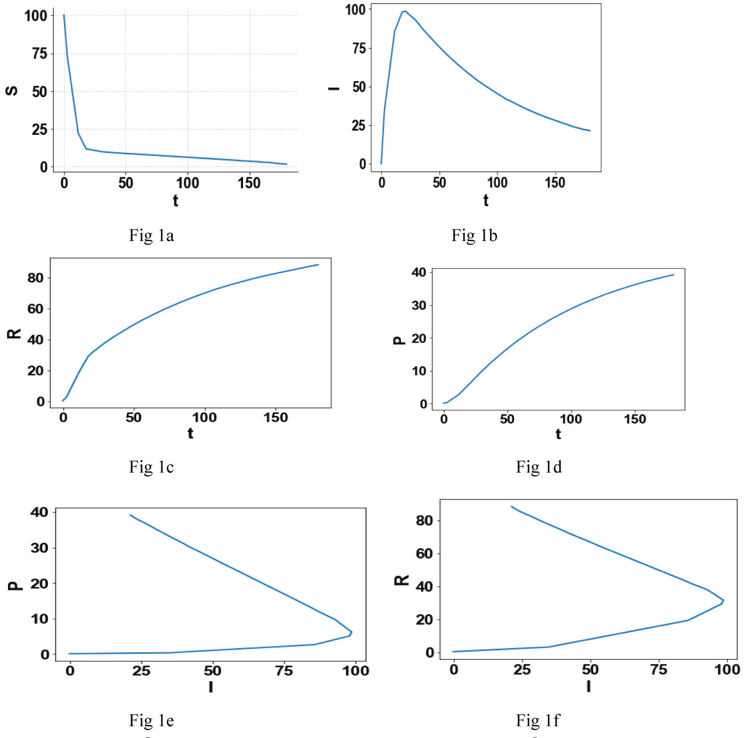 Figure 1: (a-f) The optimization results from OPTCON1.
Notice that in the 2 figures Figure 1e and Figure 1f, there is a turning point and for one value of I 2 values of R and P are possible.
View Figure 1
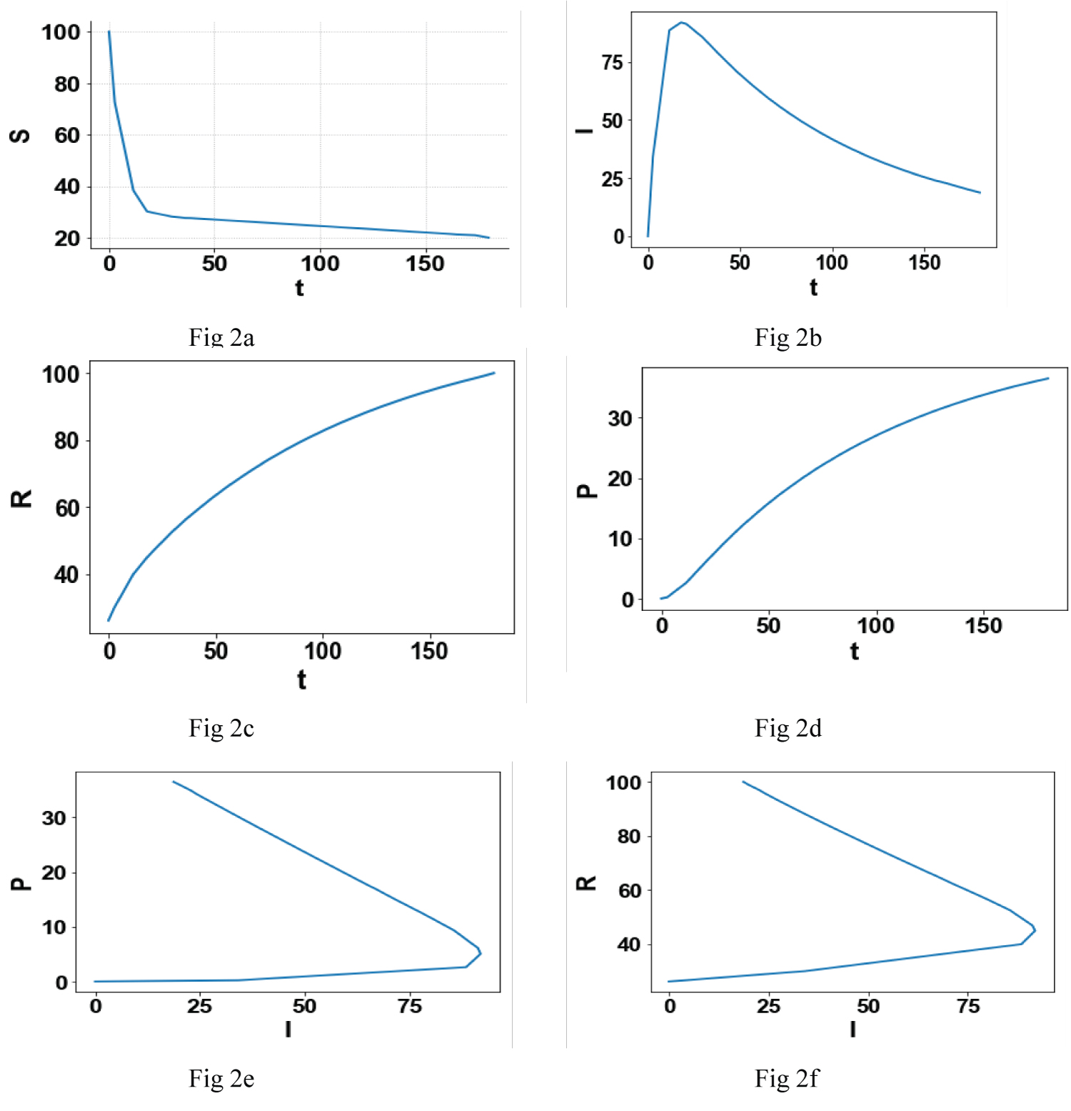 Figure 2: (a-f) The optimization results from OPTCON2.
Notice that in the 2 figures Figure 2e and Figure 2f, there is a turning point and for one value of I 2 values of R and P are possible.
View Figure 2
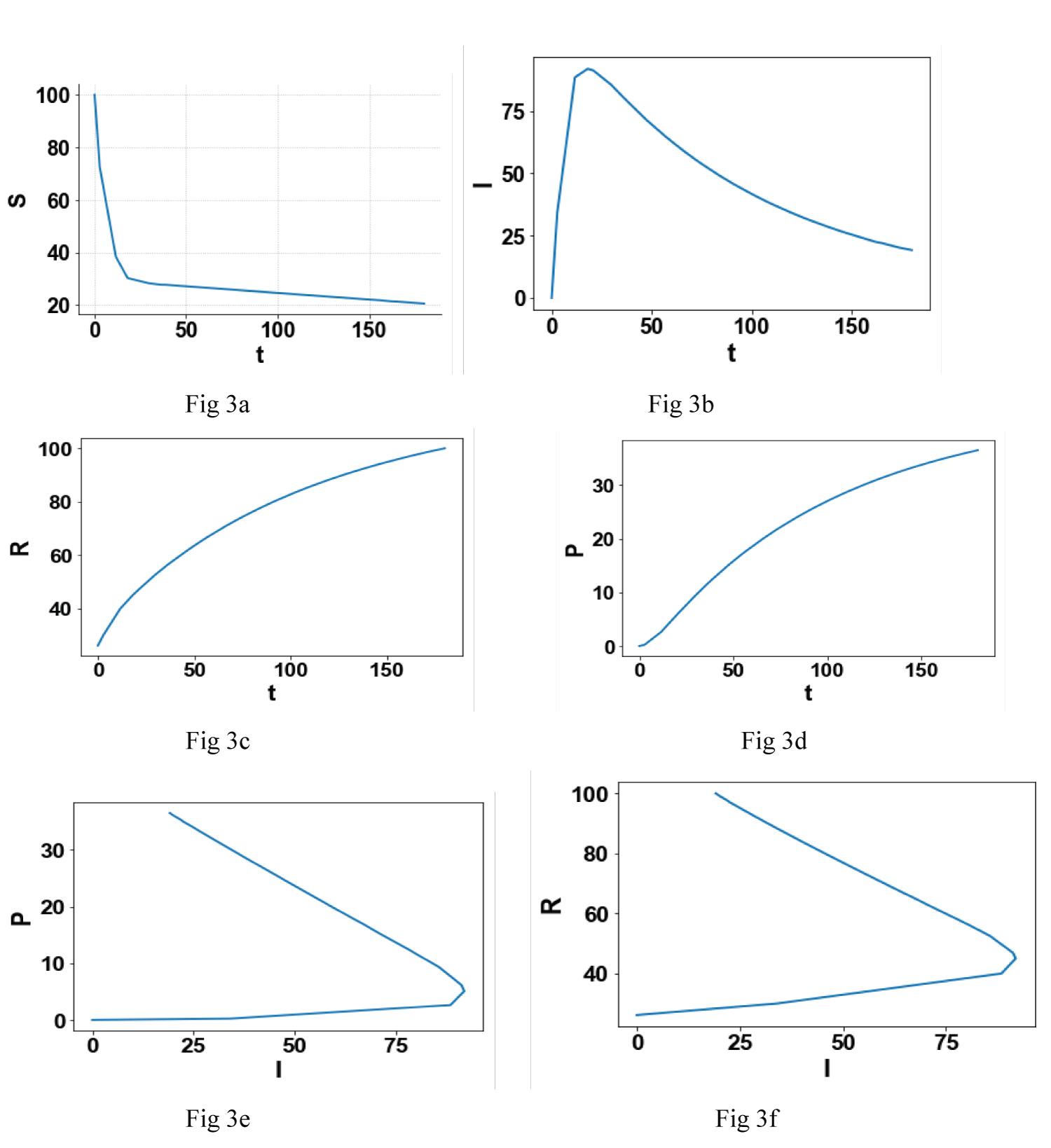 Figure 3: (a-f) The optimization results from OPTCON3.
Notice that in the 2 figures Figure 3e and Figure 3f, there is a turning point and for one value of I 2 values of R and P are possible.
View Figure 3
Figure 1b, Figure 2b and Figure 3b show that the strategies OPTCON2 and OPTCON3 result in a lower number of infected subjects than OPTCON1; Figure 1c, Figure 2c and Figure 3c show that the strategies OPTCON2 and OPTCON3 result in higher number of recovered subjects than OPTCON1 and the Figure 1d, Figure 2d and Figure 3d show that the strategies OPTCON2 and OPTCON3 result in a lower number of perished subjects than OPTCON1. The OPTCON1 strategy leads to a) Higher number of infected subjects, b) Higher number of subjects that have perished and c) A lower number of recovered subjects as compared to using the strategies OPTCON2 and OPTCON3. Hence it is preferable to use the strategies OPTCON2 or OPTCON3. There is no significant difference between the performance of the two strategies OPTCON2 and OPTCON3. However it is better to use OPTCON3 since the objective function involves more variables than OPTCON2.
A comparison of the Figure 1e and Figure 1f; Figure 2e and Figure 2f; and Figure 3e and Figure 3f demonstrate that for one value of I (infected) subjects two values of R (recovered subjects) and two values of P (perished subjects) are possible. This is an important fact because it gives the health officials the opportunity to take steps that, for a given value of I, can keep the value of R higher and the value of P lower and consequently saving lives.
The main results of this paper indicate that in trying to control the COVID pandemic, minimizing the rate of exposure to virus from infected subjects, rate exposure to virus from asymptotic/unconfirmed subjects and maximizing the rate at which unconfirmed cases become confirmed is less beneficial than minimizing the number of subjects infected I and the number of subjects perished while maximizing the number of subjects that have recovered. It is demonstrated that two values of the number of subjects recovered or perished is possible for the same value of the number of infected cases. This can enable us to take steps to ensure that less people perish and more people recover.
Dr. Sridhar thanks Dr. Saif R Kazi of CMU for his help with the graphics.