The aim of this study is to determine whether the potential toxic copper element values measured in soils (X1), vegetables (X2) and waters (X3) have an effect on the copper elements in the stomach and intestinal tissue (Yi) (ppm) of individuals in an area of approximately 2400 km2 covering the east of Erciyes strato volcano.
We applied Diamond's fuzzy least squares (FLS) method, which assumes that the deviation between the observed and the predicted values is due to the fuzziness of the coefficients. We calculated many uncertainties and errors during the calculation of the estimator of each coefficient of the model based on the minimum blur criteria.
The turbidity level of the model, which was created with an approach of h = 0.5 tolerance level, was calculated as Z(x) = 74104. Goodness of fit test criteria of fuzzy model were calculated with the mean squared error (Mean Squared Error, MSE = 47), the square root of the mean squared error (Root Mean Squared Error, RMSE = 22) and the coefficient of determination (R2 = 0.02).
As a result of the calculations, statistically, rTissue-Soil = 0.5, rTissue-Vegetable = 0.3, rTissue-Vater = 0.1 levels were determined between the potential toxic copper elements in the soil, vegetables and water and the potential toxic copper element value in the stomach and intestinal tissue. Applications to determine whether there is a relationship between potential toxic copper elements related to the study area and potential toxic copper element value in stomach and intestinal tissue are discussed for the first time in this study.
Human tissue, Copper, Fuzzy least squares regression, Volcanic soils
The products of the volcanic activity are the source for potentially toxic elements (PTE) such as As, Hg, Al, Rb, Mg, Cu and Zn [1]. The soils formed on volcanic materials including high amounts of PTE are found in many regions of the world [2]. The factors controlling to the total and biologic available concentrations of the PTE in soils are very important for human toxicology and agriculture production [3]. The distribution and amount of PTE in soils depends on the nature of soil material, weathering processes, bio cycling and addition from atmosphere and deposition from natural resources [4]. These events influence soil development and the mobility of specific elements, including PTE, in the soil system. The weathering and in-situ alteration of rock-forming minerals are one of main natural sources of PTE to the soil system and metal concentrations in soil can generally be predicted from the element concentrations in the parent material [5].
Potentially toxic elements in the structure of soil main materials enter the structure of soils with the formation of soils. These potentially toxic elements reach vegetables, surface and groundwater through plant roots and pollute the entire ecosystem. When people living in these ecosystems use vegetables, fruits and juices contaminated with potential toxic elements, they take them into their bodies.
When potentially toxic elements are taken into the human body, they cause destruction and diseases in the organs that are first digested, some suppress cell production in the bone marrow (lead), some cause cancers (arsenic), some cause metabolic problems and fatigue, some cause rheumatic problems, some cause immune system diseases, there are many clinical studies [6] showing that it causes behavioral disorders due to psychological and neurological effects. In a comprehensive study conducted in America in 2004, it was found that the fetus had heavy metals in the intraverine period in blood samples taken from newborn babies [7].
Some of the potential toxic elements accumulating in the human body are copper, zinc, lead, cadmium, mercury, aluminum, nickel, cyanide, chromium, arsenic, cobalt, uranium, magnesium, manganese. Few studies have investigated the relationships between vegetables and juices containing these potentially toxic elements and potential toxic elements in the human body. Türkdoğan, et al., [8] reported that PTE contents (Co, Cd, Pb, Zn, Mn, Ni, Cu) in soil, vegetables, and fruits in Eastern Turkey were 2-340 times higher than standard values. Several dietary contaminants (nitrates, nitrites, polycyclic hydrocarbons, alpha toxin) and environmental factors (PTE and radioactivity) play important roles in the pathogenesis of upper GI Ca [9]. Several studies revealed the carcinogenic effects of several PTEs such as Cd, Co, Cr, Ni, Pb, As, and Se [9,10].
Volcanic and volcaniclastic rocks cover a significant part of Turkey. The majority of these rocks are located in the Volcanic Province of Cappadocia (VPC) (300 × 60 km about 18000 km2). The soils located in this province were formed on volcanic parent materials of Neogene-Quaternary ages. Volcanic activity causes the release of PTEs such as As, Hg, Al, Rb, Pb, Ni, Co, Cr, Mg, Cu, and Zn, which in turn cause water and soil pollution. Ni, Co, and Cr concentrations in andesitic parent material from the Erciyes strato volcano were found to be between 48-106 ppm, 22-52 ppm, and 65-201 ppm, respectively [11].
In this study, it is aimed to estimate how much of copper (Cu), one of potential toxic elements in naturally occurring soils on the main materials sprayed from Erciyes Strato Volcano, is passed to vegetables consumed, water used for agriculture and drinking and people. Fuzzy least squares regression analysis approach was used to determine the relationships between copper (Cu) values (Yi) (ppm) in tissues and copper values in soils (X1), vegetables (X2) and water (X3). The subject of this study is to determined the relationships among copper in the soil, vegetables, fruits and human tissue using least squares regression analysis approach.
The research was carried out in an area of 2400 km2 (60 km × 40 km) east of the Erciyes strato volcano (Figure 1c). The stratified random sampling method reported by McGrew and Monroe [12] was used in the study. The points where the samples will be taken are divided into layers using the index maps produced from LANDSAT-ETM + satellite image, existing digital earth maps with 1/25000 scale (KHGM, 2002) and 1/250000 scale digital elevation model [13]. Thus, the location of the area in which the study will be carried out in Kayseri province (Figure 1a), the heightening stratification with 250 m intervals (Figure 1b) and the sampling points determined by considering the layers described above (Figure 1c) [14] determined.
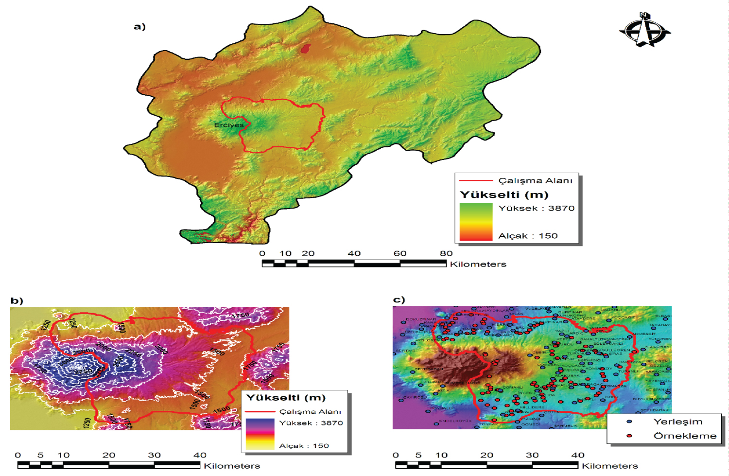 Figure 1: The location of the study area in Kayseri province (a), elevation stratification created in the 250 m elevation range (b), Geographic distribution of the soil samples from the study area (c) [15].
View Figure 1
Figure 1: The location of the study area in Kayseri province (a), elevation stratification created in the 250 m elevation range (b), Geographic distribution of the soil samples from the study area (c) [15].
View Figure 1
After entering the sampling points that GPS device form the subject of the research, a total of 330 soil samples were taken from 3 different depths (0-30, 30-60 and 60-90 cm) of each sampling point (Figure 2).
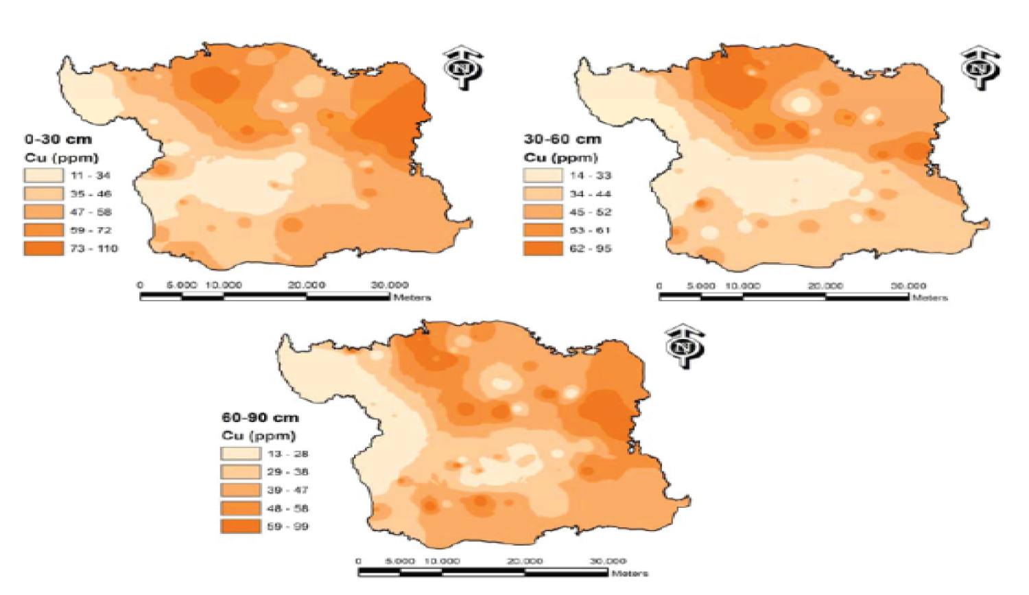 Figure 2: Spatial distribution of copper (Cu) values at three different depths [15].
View Figure 2
Figure 2: Spatial distribution of copper (Cu) values at three different depths [15].
View Figure 2
Tissue samples were taken from stomach and intestinal tissue of 36 patients who applied to Erciyes University Medical Faculty with the possibility of gastric and intestinal cancer living in the study area.
Fuzzy least squares regression analysis method was used to determine the relationships between copper (Cu) values (Yi) (ppm) in tissue samples and copper values in soils (Cu) (X1), vegetables (Cu) (X2) and waters (Cu) (X3). Estimated mean values and propagation values of copper values in gastric and intestinal tissue, which are accepted as dependent variables, and fuzzy statistical values such as confidence intervals of these values were calculated. One of goodness of fit test criteria used to determine the validity and reliability of the fuzzy least squares regression analysis model, Mean Squared Error (MSE) of errors, square root of mean square error (Root Mean Squared Error, RMSE) and coefficient of determination (R2) were calculated with the criteria values. For the analysis of these data, EXCEL 2016, LİNGO 16.0 and SPSS for WINDOWS Version 24.0 package programs were used.
Classical regression analysis methods have many useful applications. However, problems arise in a wide variety of situations, such as small data sets, differences between assumptions about distributions, relationships between dependent and independent variables, and uncertainties in the occurrence of events and inability to rank these uncertainties [16].
For these and similar situations, the values representing the data are aimed to be better represented by values in the range number type rather than a single measurement value [17]. Especially, when the boundaries of the range number type statistics cannot be determined precisely, the theoretical foundations of fuzzy set theory are used [18]. Fuzzy least squares regression analysis approach explains fuzzy functional relationship between dependent variables and independent variables with feasibility and fuzzy set theory [19].
In order to create fuzzy least squares regression analysis equation, n pair (yj, xj1,..., xjn) j = 1 ,..., m, consisting of observation values, p-1 n units, Xij = [xj1, xj2, ..., xj(p-1)]t j = 1, 2, ..., p-1, i = 1, 2,.., n, a sample dataset explained with observed independent variables and a single dependent Yi variable is considered [20,21]. In cases where there are definite independent (explanatory) observation values, the fuzzy multiple linear regression analysis equation conformed with the least squares method is usually defined by;
[22,23]. In applications performed with fuzzy regression analysis equation, the extent to which the independent variable or variables affect the dependent variable is measured by the coefficients of the variables. In order to calculate the values of the estimated fuzzy coefficients of Equation 1 with the least squares method,
the total squares between the observation values and the predicted values Minimize should be reduced to a minimum level according to Equation 2 [4,16-19].
It is possible to analyze the relationship between variables with the analysis model created as a result of providing this condition [16,18,24].
Analysis of the model coefficients based on minimum turbidity tolerance levels, the analysis of the matrix system as is as follows [16,25].
n: Number of observations, p: Number of arguments;
Here; refers to the dependent variable, estimated as a fuzzy number, and is denoted as represents the mean value (center) and denotes the spread value. [Y1,Y2,...,Yn]T the (n × 1) dimensional dependent (explained or predicted) variable vector of the i sample is assumed to have a certain error i = 1, 2, 3, ..., n.
The data of the dependent variable estimated in the fuzzy least squares regression model can be an exact or fuzzy number. Generally, if the coefficients are fuzzy and independent variables are absolute numbers, the data of the predicted dependent variable is assumed to be fuzzy numbers in the range number type [26].
The exact values of n × p-sized i, for example, j independent (explanatory) variables are vectors; used to estimate the value of the dependent variable (j = 1, 2, ..., p-1) [27,28]. It is a vector representing (p × 1) size unknown coefficients.
The coefficients vector in the function is a triangular fuzzy number (Triangular Fuzzy Numbers) and explained as = (cj,sj) ≥ 0, (j: 0, 1, 2, 3, ...., p-1). cj: Shows center value, sj: Shows spread value [25,27].
The propagation values of the fuzzy coefficients are calculated as,
with the constraints in equation 4 and equation 5 [20,25,29]. The differences between the calculated fuzzy coefficients and and values of the model are reduced to a minimum [21].
The equality of the goodness of fit test criteria used to check the validity and reliability of the models created by the approach is given below [12,13];
✔ Mean Squared Error (MSE),
✔ Root Mean Squared Error (RMSE),
✔ Determinaton Coefficient (R2),
Determination of valid and reliable models with test criterion criteria in these equations has been realized. Here n: Shows the number of observations, yi: Observed values, Shows the estimated values vector in n × 1 dimension and Average of observed values.
Depending on the copper values in soil, vegetable and water samples, fuzzy least squares regression analysis and classical least squares regression analysis method were applied to show that the copper values taken from the stomach and intestinal tissue of 36 patients can be estimated with minimum error. Comparison was made according to the fit indexes such as MSE, RMSE and R2 calculated as a result of these applications.
The data of the copper values taken from the stomach and intestinal tissue of 36 patients and the data of the copper values in the soil, vegetables and waters were obtained as in Table 1. The copper values in the tissues ranged from 825 to 3130, the copper values in the soil ranged from 9 to 146, while the copper values in vegetables ranged from 53 to 165, while the copper values in the waters did not change.
Table 1: Sample data set of copper values from 36 stomach and intestinal tissue and Cu values in soil, vegetables and water. View Table 1
Some parameter values required for the classical least squares regression analysis Equation (9) are summarized. = 1090.225 - 0.132xi1 + 2.661xi2 + 790.096xi3 + εi, i = 1, 2, ...., 36 (9) equation was achieved.
Regression was statistically significant in the analysis of variance for this equation (p < 0.01). With the equation (9), it was concluded that, the part of a coefficient size of 790.096 of the copper values in the stomach and intestine tissues of 36 patients is water-sourced, and a part of the
coefficient size such as 2.661 is from vegetables. Soils were determined to have a reducing effect. The reason for the negative copper values in the stomach and intestinal tissues is that the copper contents of the soils formed on the main materials of Andesite and Tuff were statistically negative. The variation width of the copper values observed in the stomach and intestinal tissues was between 1355-1739, while the variation width between the equation (9) and the estimated copper values was found between 1318-1559 (Table 2). According to these calculated results, the change between the estimated values was found to be less than the change between the observed values.
Table 2: Statistics of the estimated copper values in the stomach and intestinal tissue of 36 patients with the classical least squares regression analysis approach View Table 2
There is no statistically significant difference between the Cu values observed in the tissue and the mean of the Cu values measured in the tissue.The common coefficient of variation between the Cu values observed in the tissue and the Cu values estimated in the tissue was found to be 27.07. There is a weak correlation between the Cu values observed in the tissue and the Cu values estimated in the tissue (Figure 3).
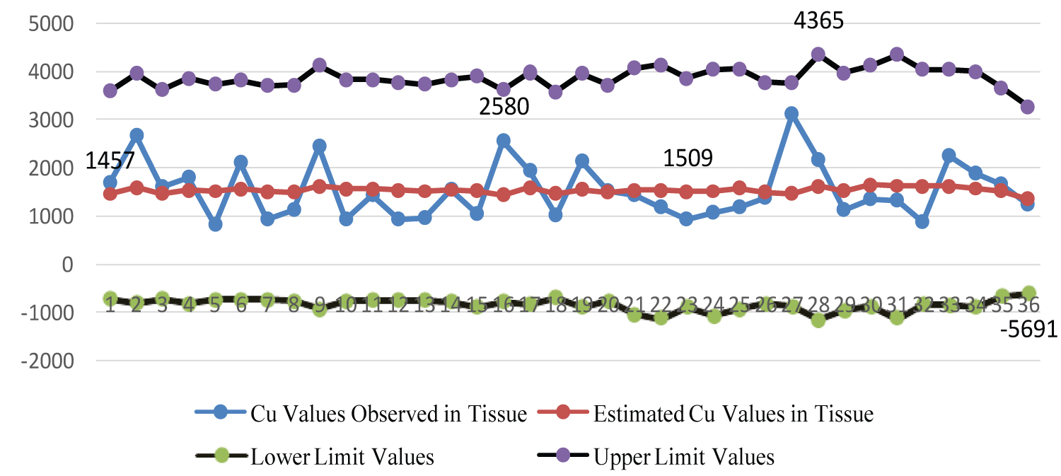 Figure 3: Graphical representation of the lower and upper limit values of the estimated Cu values observed in the stomach and intestinal tissue by classical least squares method.
View Figure 3
Figure 3: Graphical representation of the lower and upper limit values of the estimated Cu values observed in the stomach and intestinal tissue by classical least squares method.
View Figure 3
The degree of agreement between the Cu values observed in the stomach and intestinal tissues and the estimated average Cu values was statistically very low (Figure 4).
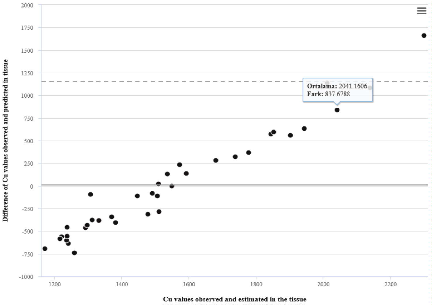 Figure 4: The degree of compatibility between the Cu values observed in the stomach and intestinal tissue and the estimated Cu values.
Fit index values were calculated as MSE = 823.70, RMSE = 28.92 and R2 = 0.0171.
View Figure 4
1) Using the copper values taken from the stomach and intestinal tissue of 36 patients and the copper values in the soil, vegetables and water, the fuzzy least squares regression analysis approach proposed by Diamond in 1988 was applied to the sample data set in Table 1 according to the following sequence of operations. The center values (cj) and diffusion values (sj) of the coefficient values j = 0,...3. of the regression analysis equation which belongs to the fuzzy least squares calculated at h = 0.5 turbidity tolerance level values were obtained
2) h = 0.5 Fuzzy least squares regression analysis equation created using coefficient values calculated at the turbidity tolerance level was created as
= (3753.4; 1029.22) + (0.14; 0.00)Xi1 + (-4.93; 0.00)Xi2 + (-7608.78; 0.00)Xi3 (12)
It is concluded that the part of the coefficient values in the Equation (12) formed, which is the size of a coefficient of (0.14; 0.00), is caused by soil, while the part caused by vegetables (-4.93; 000) and the part caused by water (-7608.78; 0.00) and has a decreasing effect.
3) System turbidity value of fuzzy least squares regression resolution equation in Eq. 12 is calculated with Z(x)
z = 2[36 × s0 + 1779 × s1 + 4202 × s2 + 7 × s3] (13)
z = 74104 as the goal function.
4) With the equation (12), the estimated mean copper values in the stomach and intestinal tissue of 36 patients in Table 1 and lower turbidity limit values and upper turbidity limit values were determined (Table 3).
Table 3: h = 0.5 turbidity tolerance in the tissue estimated average statistics for Cu values. View Table 3
There is a statistically significant difference between the Cu values observed in the tissue and the means of the average Cu values estimated in the tissue. The common coefficient of variation between the Cu values observed in the tissue and the average Cu values measured in the tissue was found to be 26.14. No statistically significant relationship was found (Figure 5 and Figure 6).
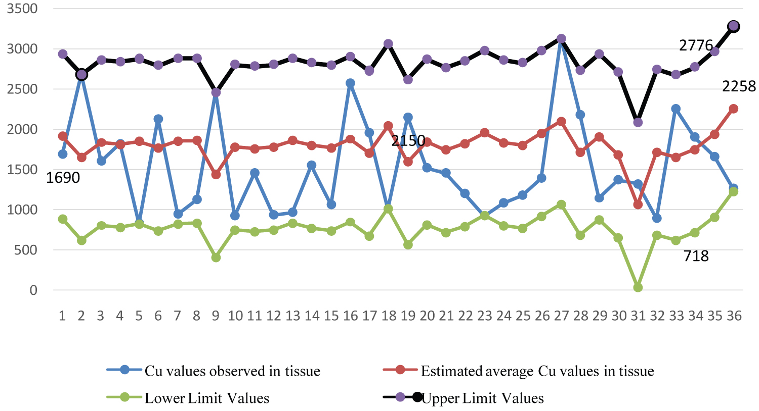 Figure 5: Graphical representation of lower and upper turbidity limit values of mean
Cu values observed in the stomach and intestinal tissue.
View Figure 5
Figure 5: Graphical representation of lower and upper turbidity limit values of mean
Cu values observed in the stomach and intestinal tissue.
View Figure 5
 Figure 6: Degree of compatibility between Cu values and estimated average Cu values observed in stomach and intestinal tissue.
View Figure 6
Figure 6: Degree of compatibility between Cu values and estimated average Cu values observed in stomach and intestinal tissue.
View Figure 6
As a result of the measurement, it has been determined that there is a low level of harmonization relationship between the values obtained and the estimated values at the level of h = 0.5 turbidity tolerance such as 0.02. Fit index values were calculated as MSE = 26.4, RMSE = 5.5 and R2 = 0.02.
Gastro-intestinal cancer (GI Ca) is a common global malignancy, accounting for twenty five percent of all cancer-related deaths [30]. Esophageal and gastric cancers are the leading malignancies in the geographical belt that extends from the Far East to the Near East, including Turkey [31]. The poor socio-economic conditions are one of the many environmental risk factors related to the development of upper GI Ca in the so-called 'cancer belt'. The potential cancer risk regions have barren lands, high mountainous areas, and soil rich in PTEs. Epidemiological studies have revealed the high prevalence of systemic cancers, especially GI Ca, in the regions where PTEs, radioactive elements, and their derived products are ubiquitous in an environment polluted with industrial and agricultural waste [32,33].
Whether there is a relationship between the copper (Cu) values in the tissue and the copper values in the soil (Cu), vegetables (Cu) and water (Cu), fuzzy and classical least squares were calculated by regression analysis methods. There was no statistically significant relationship in the results obtained from the two methods.
With different regression models, it can be said that the transport rates of copper values carried by soils, vegetables and waters change according to uncertainty level. In addition, a statistically significant relationship rTissue-Soil = 0.48, rTissue-Vegetable = 0.32, rTissue-Water = 0.12 was no found between the potential toxic copper element in the stomach and intestinal tissue and the potential toxic copper element values taken from soil, vegetable and water samples. Based on these relationships, it can be not said that gastric and intestinal cancer disease occurs due to the potential copper toxic element taken through soil, vegetables and water.
This study was supported by The Scientific and Technological Research Council of Turkey, project TUBITAK CAYDAG 106Y307.