Monthly tuberculosis (TB) counts from January 2001 to December 2018 showed an upward trend (data from SINAN - Information System for Notifiable Diseases). The increase in the incidence of TB in general is associated with an increase in the rate of extreme poverty, an increase in AIDS cases and other factors. Combining the polynomial linear regression and stochastic volatility models, the purpose of this study was to analyze monthly count data as well as the AIDS/TB, extreme poverty/TB and urban/TB rates associated with the incidence of TB. The results were obtained using the Monte Carlo method in Markov chains under a Bayesian approach. In analyzing the data with the presence of great volatility, despite the growth of TB cases in Brazil, some rates such as AIDS/TB and extreme poverty/TB are decreasing in the same period, indicating that TB cases have increased in the last few years for all sectors of the population of Brazil. The proposed model can be of great use for other epidemiological data, in addition to modeling TB counts and rates associated with TB.
TB count, Polynomial regression models, Stochastic volatility models, Bayesian methods, MCMC simulation
Tuberculosis (TB) is an infectious disease, caused by Mycobacterium tuberculosis. The disease is usually presented as pulmonary TB, but it can also affect other organs (extrapulmonary TB). Tuberculosis usually progresses slowly from the latent phase (infection without active disease, LTBI-Latent Tuberculosis Infection) to active TB, except in HIV-infected patients where the progression can be rapid and fatal. Only a small proportion (5% to 10%) of people infected with M. tuberculosis progress to active TB as reported by the [1]. Despite great scientific advances, the evolution of treatment and the discovery of a vaccine have contributed to the control of TB, it is still among the infectious diseases of high lethality in the world. Global trends show that the incidence of tuberculosis (TB), prevalence and mortality rates are gradually decreasing worldwide. TB counts in all countries and regions of the world were in great decline until the early 1980's when the first cases of patients infected with the HIV virus leading to AIDS emerged and consequently leading to a large increase in the incidence of TB in the World. After the discovery of new therapies against HIV, TB counts started to drop in practically all countries. Tuberculosis remains a poverty-related disease with a high burden of disease in low- and middle-income countries and in countries with a high incidence of HIV [2].
In Brazil, especially with the great economic crisis from the years 2014 with the increase of unemployed workers and significant increase of individuals living in extreme poverty, a new trend of increase in TB cases has been observed, regardless of the increase in AIDS cases. Many studies related to the count of individuals diagnosed with TB have been published in the literature in Brazil and in other countries.
In this direction [3], analyzed some estimates made by the WHO and indicators of incidence, mortality, occurrence of multidrug resistance and association with HIV for tuberculosis in Brazil and worldwide. These authors present estimates (8.7 million new cases per year in the world and 116,000 new cases per year in Brazil) or actually verified (Brazil in 2000 notified 82,249 new cases) pointing out to a serious public health situation, mainly in developing countries, which it requires energetic and effective measures for its control. In a country of high prevalence like Brazil, the actions for the discovery of new cases, associated with the measures of biosafety, are of interest to all health professionals, mainly those who work in large hospitals or emergencies.
DC Costa [4] analyzed several aspects that influence the pattern of tuberculosis mortality and morbidity: The variation in living conditions, the effects of chemotherapy and the dynamics of disease transmission which characterizes the indicators used in the measurement of tuberculosis that are built from prevalence surveys and notification data. The main indicators are: risk of infection, mortality, incidence coefficient of tuberculous meningitis, incidence coefficients of tuberculosis cases, especially pulmonary bacilliferous among others. In that study, data on the incidence of bacilliferous pulmonary cases in the Brazilian provinces of Pará and Rio Grande do Sul and mortality from tuberculosis in the capitals of Pará, Rio Grande do Sul, Pernambuco and Rio de Janeiro were analyzed, which reveal in general, a downward trend at that time, still that at a different pace.
Many other studies are presented in the literature. LMW Acosta, et al. [5] relate some social determinants and the incidence of TB in Porto Alegre, RS, Brazil. Several recent studies consider different statistical models that capture temporal or spatial effects in the analysis of TB epidemiological series [6-12].
Some studies on the incidence of TB have used ARIMA [13] time series models (autoregressive integrated moving average models) or ARCH [14] models (autoregressive conditional heteroscedasticity) in the analysis of epidemiological series. In this sense, RR Sarkar, et al. [15] consider the application of different time series models for epidemiological data with application to malaria. YL Zheng, et al. [16] use ARIMA models and a combination of ARIMA-ARCH models for predicting and monitoring monthly tuberculosis morbidity in Xinjiang, China. In this case, the ARCH model is suggested to provide tuberculosis surveillance, providing estimates on tuberculosis morbidity trends in Xinjiang, China. Other applications in epidemiology can also be seen in [17-25].
In the present study, a new formulation of statistical modeling (combination of polynomial linear regression models with stochastic volatility models) is proposed for the analysis of TB count data and associated rates using Bayesian methods of statistical inference. The article is formulated as follows: in section 2 the monthly data on TB in Brazil for the period 2001 to 2018 are presented; section 3 presents the material and methods; section 4 presents the obtained results; finally, section 5 presents conclusions and discussion of the obtained results.
This study considers TB count data in Brazil between the years 2001 and 2018 and some existing relationships given by other time series in the same period such as rates of AIDS patients among patients diagnosed with TB, rates of patients living in urban centers among patients diagnosed with TB, rates of male patients among patients diagnosed with TB, rates of patients in extreme poverty among patients diagnosed with TB among several other factors. Figure 1(a) shows a graph of the yearly time series of TB patient counts in Brazil (data from the SINAN-Information System for Notifiable Diseases-http://sinan.saude.gov.br/sinan/login/login.jsf) for the period between January 2001 and December 2018 (data set in Appendix 1 at the end of the paper). Figure 1(b) also shows the rates (number of TB cases in the year divided by the estimates of Brazil's population in the year, source IBGE). The data are presented in Table 1, from where it is observed an increase in TB rates between the years 2001 and 2003; from 2003 onwards there was a decline in yearly TB rates until 2016, possibly due to the efficacy of drugs to control AIDS; after that year, an increase in TB rates is observed again, perhaps as a result of the great economic crisis affecting Brazil (increase in extreme poverty, increase in the unemployed rates, lower investments in health, among many other factors). From Figure 1, it is observed two change-points: One change-point around 2003 and a second change-point close to the year 2017.
 Figure 1: Yearly counts of TB patients in Brazil and yearly rates per 100,000.
View Figure 1
Figure 1: Yearly counts of TB patients in Brazil and yearly rates per 100,000.
View Figure 1
Table 1: Yearly counts of TB patients in Brazil and yearly TB rates. View Table 1
Figure 2 shows the monthly TB counts in Brazil (data from SINAN) from January 2001 to December 2018 (216 months). From the graphs presented in Figure 2, it can be seen that:
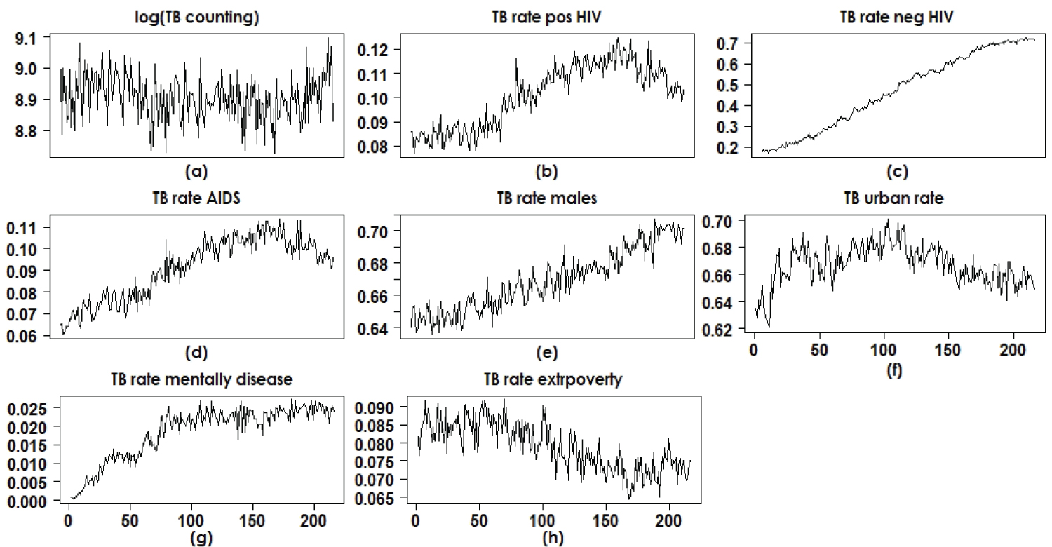 Figure 2: Time series of counts and rates of TB patients in Brazil.
View Figure 2
Figure 2: Time series of counts and rates of TB patients in Brazil.
View Figure 2
• The monthly counts of patients diagnosed with TB in the period between January 2001 and December 2018 (original scale and logarithmic scale) show seasonality for the seasons and there is clearly a yearly decrease in counts until the year 2014 where the beginning of an increase in TB cases is observed.
• It is also observed that until the mid-2014 there is a tendency to increase the rates of AIDS patients among TB patients; in that year there is a beginning of a decrease in the rates of AIDS patients among those infected with tuberculosis. This is also seen for rates of HIV-positive patients among TB patients. It is important to note that the incidence of TB was in great decline worldwide until the mid-1980s, the year of the beginning of the AIDS epidemic, a factor that led to the reappearance of TB in large numbers. From these graphs it is possible to conclude that there is a strong indication of the increase in TB in Brazil for all segments of the population regardless of the effect of HIV, as the rates of HIV-infected patients diagnosed with TB are declining, despite the increase in TB cases.
• It is also observed that the rates of urban patients among those infected with TB had an annual increase until mid-2012; as of that year, there has been a decline in the number of patients living in urban centers (people most susceptible to HIV infection) among TB patients. This also shows that the incidence of TB is gradually increasing for all segments of the population in Brazil, a result of great serious impact to the Brazilian heath authorities. The same is observed for patients in extreme poverty (annual decrease in the rates of individuals in extreme poverty among TB patients).
Figure 2 shows, in most cases, for the data analysis and statistical data modeling, the need for polynomial linear regression models in the presence of the covariate (independent variable) month (temporal order) that can capture possible effects of linearity and that also have regression coefficients associated with quadratic and cubic effects. A quadratic term or cubic term transforms a linear regression model into a curve. Since the regression model has the covariate month squared or cube, and not the regression coefficient, the model remains a linear regression model [26,27]. An application of polynomial regression models with epidemiology data is given by [28]. The presence of a quadratic term in the model creates an inverted U- or U-shaped curve, as seen in the graphs in Figure 2(b), Figure 2(d), Figure 2(f), Figure 2(g) and Figure 2(h). A cubic term has two distinct parts: one facing up and one facing down, that is, the curve goes down, back up and back again (or vice versa). This is also seen in some graphs in Figure 2(a), Figure 2(c) and Figure 2(e).
The main goals of the study are:
• To model the monthly TB counts in Brazil with data on the logarithmic scale from 2001 to 2018, assuming stochastic volatility models to estimate the time series volatilities;
• Also to model some rates of factors associated with the incidence of TB using stochastic volatility models such as rates of patients diagnosed with TB and AIDS, rates of patients diagnosed with TB and urban dwellers and rates of patients diagnosed with TB and belonging to the socioeconomic groups of extreme poverty.
• To study the variability in the rates of patients diagnosed with TB and AIDS, rates of patients diagnosed with TB and residents of urban centers, rates of patients diagnosed with TB and belonging to extreme poverty socioeconomic groups that are decreasing despite the growth of TB cases seen in Brazil in recent years.
• To model yearly TB rates in Brazil from 2001 to 2018, assuming linear regression models in the presence of change-points.
In a first data analysis, it is assumed a standard polynomial linear regression model given by:
Y(t) = βo + β1 months(t) + β2 [months(t)]2 + β3 [months(t)]3 + ε(t) (1)
for t = 1, 2, ..., 216 (months) where ε(t) are noises considered independent and identically distributed random variables with a normal distribution N(0, ). Under a classic approach, the regression parameters are usually estimated using the least squares method (EMQ). An alternative of epidemiological interest would be to model the series not only to estimate monthly averages, but also to estimate monthly variances (volatilities) that are of interest to the public health area, possibly relating these volatilities to the occurrence of non-observed factors associated with the months (season, unemployment rate, extreme poverty rate, among others). For this purpose, time series models are used in the data analysis, which simultaneously estimate the monthly average and the monthly volatility.
Stochastic volatility (SV) models have been widely used to analyze financial time series [29] as a powerful alternative to some existing regression models in the literature, such as the ARCH (conditional heteroscedastic autoregressive) models introduced by [30] and the generalized autoregressive conditional heteroscedastic models (GARCH) introduced by [31], but not widely used in the health field [32-34]. In one of these few health applications, [35] studied neural signals using a database of medial temporal lobe (MTL) recordings from 96 neurosurgical patients, using time series models with volatility described by a multivariate stochastic latent variable process and lagged interactions between signals in different brain regions providing new insights into the dynamics of brain function. In the financial area, these models are considered for modeling the logarithms of financial returns between current data and previous data (can be hours, days or months) without taking into account the modeling of the means depending on covariates.
The novelty of this study is the introduction of stochastic volatility models for epidemiological time series, in particular, for tuberculosis counting series in Brazil.
For the definition of the models, N ≥ 1 is a fixed integer that records the amount of observed data (in our case, it will represent the monthly TB counts on the logarithmic scale and also the rates of patients in certain groups among those infected with TB).
In the presence of heteroscedasticity, that is, variances depending on time t, assume that the time series Y(t), t = 1, 2, ..., N assume the combined polynomial linear regression model with the stochastic volatility model for the analysis of TB count data on the logarithmic scale and some rates related to the TB epidemic:
Y(t) = βo + β1 months(t) + β2 [months(t)]2 + β3 [months(t)]3 + σ(t)ε(t) (2)
where it is assumed that ε(t) are noises considered independent and identically distributed random variables with a normal distribution N(0, ) and σj(t) is the square root of the variance of (1) (for simplicity, we can assume = 1). The variance of Y(t) is modeled by eh(t) where h(t) depends on an unobserved latent variable.
Remark: From model (2), it is observed that:
The mean of Y(t) is given by E[Y(t)] = βo + β1 months(t) + β2 [months(t)]2+ β3 [months(t)]3 since E[σ(t)ε(t)] = 0.
The variance of Y(t) is given by var[Y(t)] = var[σ(t)ε(t)] = σ2(t) since we are assuming that var[ε(t)] = = 1.
To analyze the data set, it is introduced a latent variable (unobserved variable) defined by an auto-regressive model AR (2), for t = 1, 2, 3, ..., N (N = 216 months).
h(1) = μ + ζ(1), t = 1,
h(2) = μ + φ1[h(1) - μ] + ζ(2) (3)
h(t) = μ + φ1[h(t-1) - μ] + φ2[h(t-1) - μ] + ζ(t), t = 3, 4, ..., N,
where ζ(t) is a noise considered to be independent and identically distributed random variables with a normal distribution N(0, ), which is associated to a latent variable h(t). The quantities μ, φ1 and φ2 are unknown parameters that should be estimated (0 < φ1 < 1, 0 < φ2 < 1).
Bayesian inference procedures, based on Markov Chain Monte Carlo simulation methods (MCMC) [34,36,37] have been widely used to analyze stochastic volatility models. The main reason for using Bayesian methods is that, in general, we may have great difficulties in obtaining inferences (point and interval estimation) for the parameters of interest of the stochastic volatility model when using a standard classical inference approach. These difficulties can appear in the form of high dimensionality and likelihood function without closed form among other factors.
For a Bayesian analysis of the model (1), we assume that the prior distributions for the parameters μ, φv and ζ = v = 1, 2 are respectively given by the normal distribution, Beta(b,c) distribution and a Gamma(d,e) distribution, where Beta(b, c) denotes a beta distribution with mean b/(b + c) with variance bc/[(b + c)2(b + c + 1)] and Gamma(d, e) denotes a gamma distribution with mean d/e and variance d/e2. The hyperparameters a, b, c, d, e are assumed to be known and specified previously. Also assume that the regression parameters βj have independent normal distributions with known hyperparameters, j = 0, 1, 2, 3.
To complete the statistical data analysis of the TB counting in Brazil for the period 2001-2018 we know consider the TB yearly counting in place of the month TB counting. Considering the yearly rates of TB in Brazil, we can see (Table 1 and Figure 1) the presence of two change-points around the years 2003 and 2016 (upward rate until 2003, downward rate between the year 2003 and year 2016, rising rate after year 2016. In this case we also can use a linear regression Bayesian model to be fitted by the data in the presence of two points of change. In this case it is assumed the linear regression model,
Y(t) = βo[j] + β1[j]years(t) + ε(t) (4)
for t = 1, 2, ..., N and j = 1, 2, 3 where βo[1] and β1[1] are regression parameters for the model (data set in logarithmic scale) corresponding to time[t] ≤ ζ1 (ζ1 is the first change-point); βo[2] and β1[2] are regression parameters for the model (data set in logarithmic scale) corresponding to ζ1 < time[t] ≤ ζ2 (ζ2 is the second change-point); βo[3] and β1[3] are regression parameters for the model (data set in logarithmic scale) corresponding to time[t] ≥ ζ2 and εj(t) is the error assumed to be independently and identically distributed random variables with a normal distribution N(0, ), j = 1, 2, 3 where for time[t] ≤ ζ1, for ζ1 < time[t] ≤ ζ2 and for time[t] ≥ ζ2. In the Bayesian analysis, discrete uniform prior distributions are assumed for the change-points k1 and k2 concentrated around the years 2003 and 2016; Gamma(1,1) prior distributions for the parameters ζj = j = 1, 2, 3; βo[1] ~ N(-7,6;1), βo[2] ~ N(-7,7;1), βo[3] ~ N(-7,75;1); and β1[j] ~ N(0;0,01). We further assume prior independence.
From a preliminary analysis of the data, it is observed that in addition to the count times series for the monthly number of TB in Brazil, other series are related for the data analysis of the monthly counting of TB in Brazil from January 2001 to December 2018. In this study we consider four series in the data analysis:
• Time series for the logarithm of the TB count versus time order,
• Time series for the rate AIDS/TB versus time order,
• Time series for the rate urban patients/TB versus time order,
• Time series for the rate of patients in extreme poverty/TB versus time order.
These four series are analyzed in this section. Initially, polynomial regression models are considered in the form (1) considering constant variances and classic least squares (LSE) estimation techniques. We consider four regression models denoted by,
• Model M1: The regression model (1) associated with the logarithms of TB counts versus time order,
• Model M2: Associated with rates of patients with AIDS among TB patients versus time order,
• Model M3: Associated with rates of urban patients among TB patients versus time order,
• Model M4: Associated with the rates of patients living in extreme poverty among TB patients versus temporal order.
Table 2 shows the LSE estimators for the regression parameters of each proposed regression model obtained using Minitab® software version 17. The necessary assumptions (normality and constant variance of the residuals were verified from the residuals graphics).
Table 2: LSE for the four assumed models. View Table 2
Assuming the volatility model introduced in section 2 (equations (1) and (2)) for the four series above, also denoted here by model M1 (log (TB counts)), model M2 (AIDS / TB rate), model M3 (rate (urban patients)/TB) and model M4 (rate (extreme poverty patients)/TB), let us consider the following prior distributions for the parameters of each model:
• Model M1: φv ~ U(0,1), v =1,2; ζ ~ Gamma(1,1); μ ~ N(0,1); β0 ~ N(9,100); βj ~ N(0,1).
• Model M2: φv ~ U(0,1), v = 1,2; ζ ~ Gamma(1,1); μ ~ N(0,1); β0 ~ N(0.07, 0.01); βj ~ N(0, 0.01).
• Model M3: φv ~ U(0,1), v = 1,2; ζ ~ Gamma(1,1); μ ~ N(0,1); β0 ~ N(0.63, 0.01); βj ~ N(0, 0.01).
• Model M4: φv ~ U(0,1), v = 1,2; ζ ~ Gamma(1,1); μ ~ N(0,1); β0 ~ N(0.082,0.01); βj ~ N(0, 0.01).
Further, let us assume prior independence among the parameters. The choice of the hyperparameters for the prior distributions of the regression parameters was made based on previous knowledge obtained from the classical regression models for the regression model (1) assuming normal errors without the presence of stochastic volatility (LSE given in Table 2). In this way, empirical Bayesian methods were used [35].
In the simulation of samples for the joint posterior distribution of interest, it was used the OpenBUGS software [36], which simplifies the computational work, since this software only requires the definition of the likelihood function and the prior distributions for the parameters of the model. Thus, the conditional posterior distributions for each parameter needed for the Gibbs and Metropolis-Hastings algorithms are not presented in this study. The convergence of the sample simulation algorithm of the joint posterior distribution of interest (Gibbs/Metropolis-Hastings algorithms) was verified from time series plots of the generated Gibbs samples. It was considered a "burn-in-sample" with 51,000 samples to eliminate the effect of the initial values in the iterative method to simulate Gibbs samples for the M1 model; after this, it was generated other 120,000 samples choosing each tenth sample which gives a final sample size of 1200 to be used to obtain the posterior summaries of interest. Similarly, for models M2, M3 and M4, it was considered a "burn-in-sample" with 111,000 samples; after that, it was generated other 100,000 samples choosing each tenth sample totaling a final sample size of 1,000 to be used to obtain the posterior summaries of interest. The posterior summaries of interest (posterior means, posterior standard deviations and 95% credibility intervals) for each parameter for the four models are shown in Table 3.
Table 3: Posterior summaries for the assumed models. View Table 3
From the results presented in Table 3, it is observed that the covariate month has significant effects on the response in terms of linear effect of month (regression parameter β1), quadratic effect of month (β2) and cubic effect of month (β3) (intervals corresponding 95% credibility does not contain a zero value) for models M3 (rate (urban patients)/TB) and M4 (rate (extreme poverty patients)/TB); for the M1 model (log (TB rates)) there is a significant effect of the quadratic and cubic terms and for the M2 model (AIDS/TB rate), there is a significant effect of the linear and cubic terms.
Figure 3 shows the graphs of the observed and the fitted series assuming the models (Monte Carlo estimators of the responses mean) for the four series. A good fit is observed in all cases. Figure 4 shows graphs of the quadratic roots of the estimated volatilities.
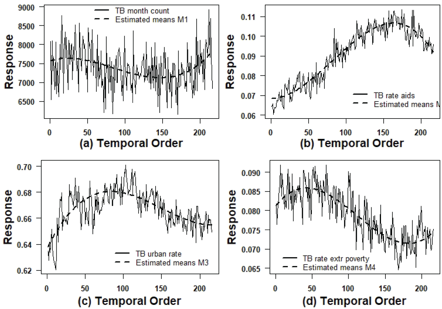 Figure 3: Graphs of the observed series and estimated means by the models.
View Figure 3
Figure 3: Graphs of the observed series and estimated means by the models.
View Figure 3
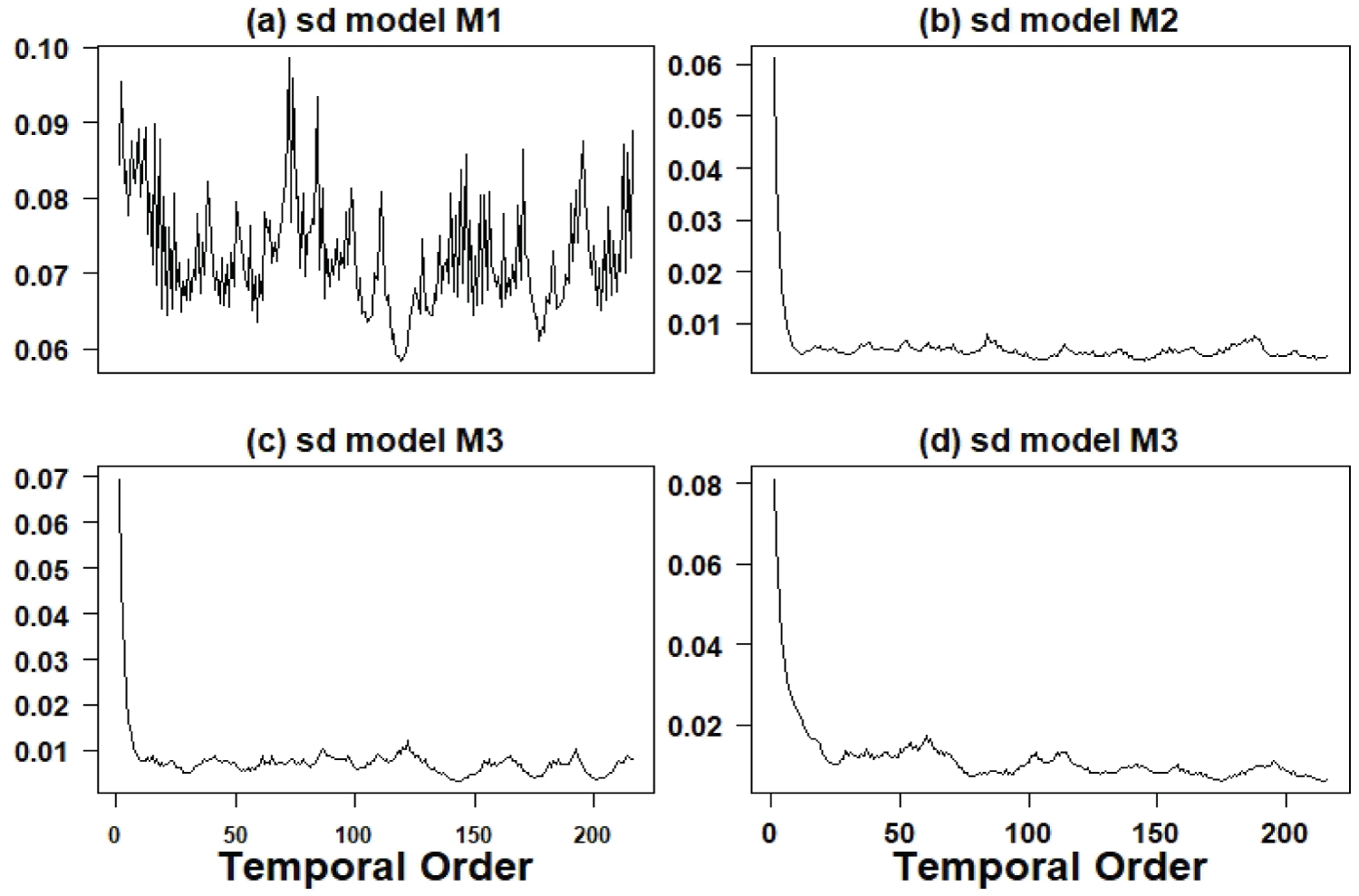 Figure 4: Graphs of the quadratic roots of the estimated volatilities.
View Figure 4
Figure 4: Graphs of the quadratic roots of the estimated volatilities.
View Figure 4
It is important to point out that from the results obtained from Table 2 and Table 3 (LSE and Bayesian estimators), it can be seen that the LSE and Bayesian estimators have close point values where in most cases related to each regression parameter, we have concordance of p-value < 0.05 and credible intervals not containing the zero value. Only for the parameter β1 (linear effect) related to models M1 (log (TB counts) versus time), and M2 (AIDS/TB rate versus time) it is observed significance under the classic approach but no significance under the Bayesian approach and for the parameter β2 (quadratic effect) for model M4 (rate (extreme poverty patients)/TB versus time), we have no significance under the classic approach and significance under the focus Bayesian we have different inferential results in terms of significant effects.
Table 4 presents the posterior summaries obtained using the OpenBUGS software (burn-in sample = 1,000; 10,000 additional Gibbs samples). Figure 5 shows the fitted model (presence of two change-points, one change-pint around the year 2003 which corresponds to the k1 estimated by 2.104 and a second change-point in the year 2016 which corresponds to the k2 estimated by 16.71). The Openbugs program code is presented in Appendix 2 at the end of the article.
Table 4: Posterior summaries for a model with two change-points. View Table 4
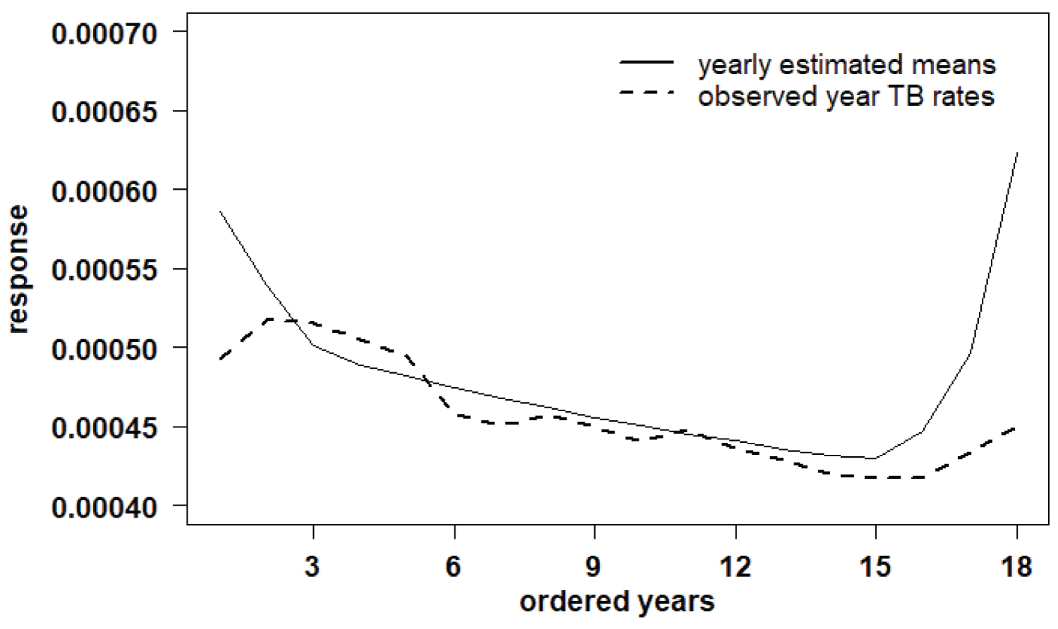 Figure 5: Fitted model (presence of two change-points).
View Figure 5
Figure 5: Fitted model (presence of two change-points).
View Figure 5
From the obtained results using model (2), it is observed a good fit of the models to the four data sets denoted here by models M1, M2, M3 and M4. Regarding to the estimated variability (volatility) of the data presented in Figure 6 for the period from July 2001 to December 2018, we have:
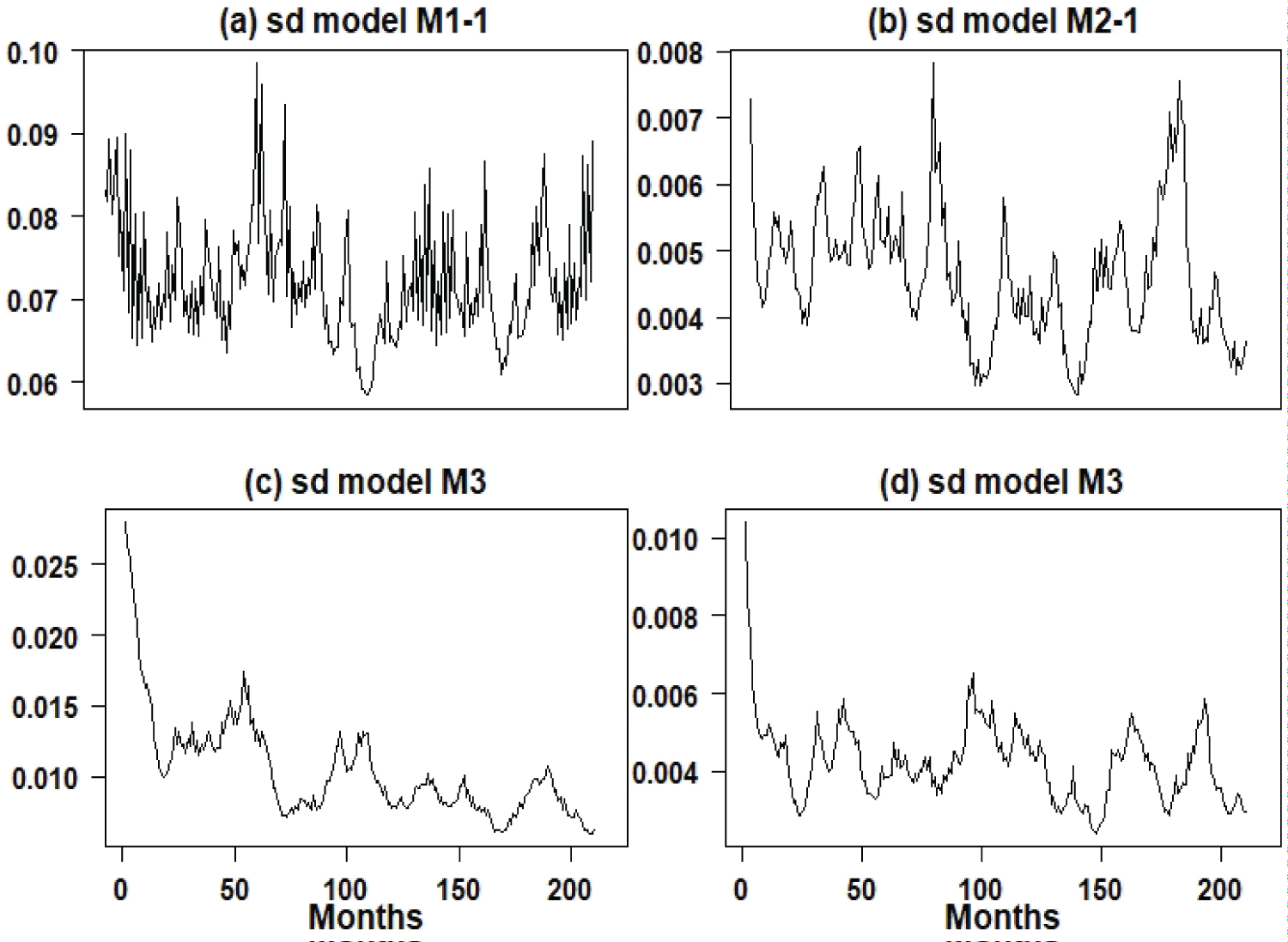 Figure 6: Graphs of the quadratic roots of the estimated volatilities (July 2001 to December 2018) for the four models.
View Figure 6
Figure 6: Graphs of the quadratic roots of the estimated volatilities (July 2001 to December 2018) for the four models.
View Figure 6
• For the TB count series considered on the logarithmic scale (model M1), there is great variability around the year 2007; from that year on, there is a decline in variability to be increased again especially at the end of the period 2001/2018.
• For the AIDS/TB rate series (model M2), there is great variability around the year 2007/2008 and 2016/2017, an indication that the AIDS/TB rate was in transition, indicating that the number TB cases were increasing regardless of whether a person have AIDS or not. It is a worrying result, as it indicates that TB is increasing in Brazil regardless of the increase in AIDS cases.
• For the urban patient/TB rate series (model M3), it is observed that the variability is declining; with this result and the lower average of urban patient/TB rates, there is an indication that the TB epidemic is increasing throughout Brazil regardless of being a resident of large cities.
• For the extreme poverty/TB rate series (model M4), it is observed that the variability is approximately stable regardless of the great seasonality with a slight decline, also indicating that the number of TB cases is increasing in Brazil, regardless the increasing of poverty; these results show that the increase in TB cases in Brazil is in a increasing phase regardless of the increase in extreme poverty that has been observed in Brazil, especially since 2019.
In conclusion, we can emphasize that the proposed model can be of great use for other epidemiological data in addition to modeling TB counts and rates associated with TB. Another important point of an epidemiological character obtained from the data analysis: As the number of TB cases is increasing in Brazil and some rates such as AIDS/TB and extreme poverty/TB are falling with the presence of great volatility, there is an indication that TB is increasing indiscriminately in Brazil, as AIDS and extreme poverty are two factors widely discussed in the literature that are associated with TB. This is a problem of public health concern.
It is important to point out, that in the present study we considered univariate epidemiological time series (modelM1 (log (TB counts)), model M2 (AIDS/TB rate), model M3 (rate (urban patients)/TB) and model M4 (rate (extreme poverty patients)/TB). Another possibility is to assume multivariate SV models and to study the structure of possible dependence among the series. This approach will be the goal of a future study.
The authors would like to thank the referee's comments that led to a great improvement in the manuscript.