Radiotherapy is a treatment of carcinogenic tumors using ionising radiation and the improvement of radiotherapy techniques has been conducted to protection of healthy tissues. Recent implementations have employed static fields with small dimensions. The interests for this work were small fields, used in modern techniques such as Stereotactic Radiation Therapy (SRS) and Intensity Modulated Radiation Therapy (IMRT). These fields have special characteristics that refer to the non-establishment of the physical conditions idealized in traditional dosimetry protocols and localized imbalances of the photon spectrum. The obtained profiles allowed to verify disturbances present in the exposures, considering the dosimetry of small fields and the impacts on the planning of local dose deposition. In this work, the dose distribution of an X-ray beam was recorded using a solid water phantom. This phantom was irradiated using small fields with 1 × 1, 2 × 2, 3 × 3 and 5 × 5 cm2. The 10 MV X-ray beam was generated in a linear accelerator model Synergy Platform from the manufacturer Elekta and radiochromic film sheets were used to record dose profiles inside a solid water phantom. The solid water phantom loaded with radiochromic film was positioned 1m away from the X-ray beam's focus. The longitudinal profile of absorbed dose obtained presented the maximum dose value at 2.24 cm of depth for both fields, inside the phantom. Smaller field size generated a maximum absorbed dose smaller. The axial dose profiles were recorded at 1 cm depth, and presented a plateau in the axis Y for the four fields. For axial irradiation on the X-axis, the central region is 99.27% in relation to 100% of the relative dose and on the Y-axis, the central region is 99.39% in relation to 100% of the relative dose.
Dose profile, Radiotherapy, Small fields, Solid water phantom
The evolutions of the radiotherapy techniques and protocols available for the treatment of cancer have introduced new theoretical and practical standards to ensure the quality and reliability of these techniques. This scope uses techniques that use small X-ray fields or even dynamic fields to achieve their goals and confer advantages over predecessors. SRS is a technique proposed by Lars Leksell based on static X-ray fields obtained through the orthovoltage unit. IMRT is a technique that uses tomographic images during the physical planning of cancer patient treatment. This type of treatment modulates the number of photons that cross a given area, modifying the beam's intensity conforming the dose to the target volume that aims to maximize the radioprotection of surrounding tissues [1-3].
Small fields are being applied in radiotherapy, include intensity modulated radiotherapy (IMRT), volumetric modulated arc therapy (VMAT), stereotactic radiosurgery (SRS), stereotactic radiotherapy (SRT) and stereotactic body radiotherapy (SBRT). The small fields are produced by the implementation of collimation tools through Cones and Multileaf Collimators (MLC) or by devices dedicated to this purpose, such as Cyberknifes and Gamma Knives. The influencing factors include finite source size, steep dose gradients, charged particle disequilibrium, detector size and associated volume averaging effects, and changes in energy spectrum and associated dosimetric parameters [4-7].
Conventionally, external-beam machines like linear accelerators with jaw or multileaf collimators (MLCs) are able to produces fields of typical dimensions smaller than 4 × 4 cm2 when being used to deliver therapeutic dose to cancer patients. A small field is understood like a field created by downstream collimation of a flattened or unflatten photon beam and differ from conventional fields in their lateral dimensions, causing penumbra areas on both sides of the field to overlap and make most commonly used detectors large in relation to the size of the radiation field. The technological development in radiotherapy, the use of increasingly smaller and/or modulated small fields generated an increase in the uncertainty of the acquisition of dosimetric data. In the literature, incidents caused by errors in the acquisition of these data from the treatment machine related to small fields have been reported [8-11].
In this work, the dose distribution of an X-ray beam was recorded using a solid water phantom. This phantom was irradiated using small fields with 1 × 1, 2 × 2, 3 × 3 and 5 × 5 cm2. The 10 MV X-ray beam was generated in a linear accelerator model Synergy Platform from the manufacturer Elekta, and radiochromic film sheets were used to record dose profiles inside a solid water phantom. The solid water phantom loaded with radiochromic film was positioned 1m away from the X-ray beam's focus.
A small field is a field having dimension smaller than the lateral range of the dose-depositing charged particles set into motion post interaction with the incident beam. With the reduction of the field, through the collimators, they can occlude the radiation source, interfering in the dose at the point where it is desired to measure, not being possible to differentiate between the primary portion of the radiation and the penumbra, because there is an overlap of the penumbra to the beam. Furthermore, in small fields the range of secondary electrons is large compared to the size of the field. Under such conditions, there is a reduction in the output factor, or beam intensity, as well as an increase in the penumbra dimension, influencing the field size of the beam to be measured. When occur dose distribution inside a planning target volume (PTV) in smaller and irregular beam lets or segments, problems arise namely lateral charged particle disequilibrium, steep dose gradients, partial occlusion of the primary radiation source by the system of collimation, detector-related field perturbations and detector volume averaging effects [3,8,12-14].
Figure 1 shows a geometric demonstration of the composition of the penumbra region. The penumbra composition in conventional fields is shown in the first drawing. In the Figure a small field was shaped by a collimator that secured part of the finite primary photon source in the produce a lower beam output on the beam axis compared to field sizes where the source is not partially blocked. This primary source occlusion is the first challenge for dosimetric studies when the field size is smaller than the size of the primary photon source.
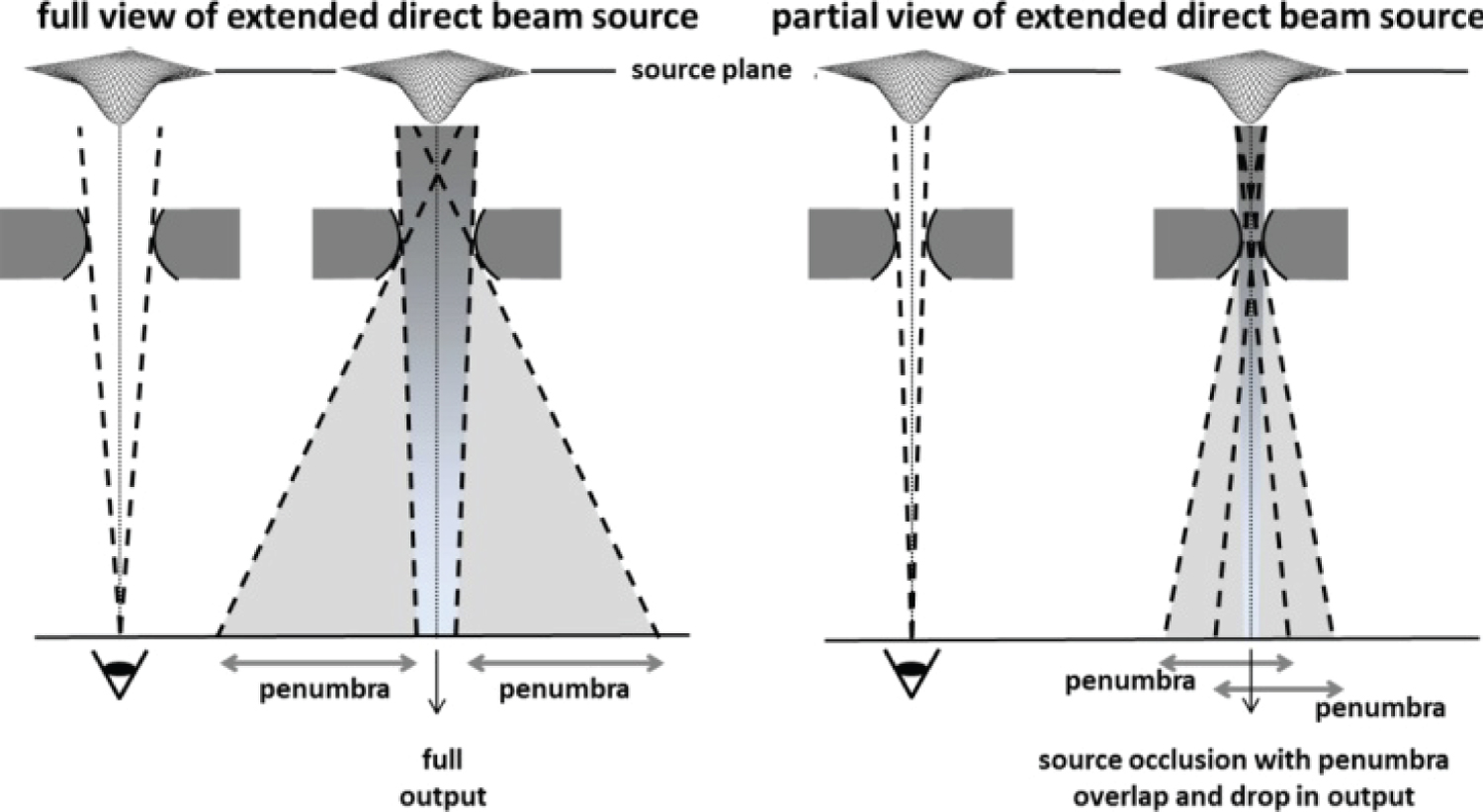 Figure 1: Schematic representation of the source occlusion effect.
View Figure 1
Figure 1: Schematic representation of the source occlusion effect.
View Figure 1
The greater obstruction of the beam causes a decrease in the homogeneity region, which makes a considerable fraction of the field composed by the beam penumbra itself. In addition to the penumbra issue, the sizing of small fields is influenced by the reach of secondary particles, since the lateral diffusion of charged particles can, according to the energy spectrum, be comparable to the field dimensions itself [6,9,15,16].
A photon beam is considered small if exists loss of equilibrium of charged particles, partial occlusion of the primary photon from the source by collimating devices or the detector size being large compared to the beam dimensions. The characteristics presented are related to the beam in overlap between field penumbras and detector volume [11,17].
Another important factor to note is in relation to the definition of the field size. In conventional fields, this is defined as the distance between the points where a given isodose curve, usually 50%, intersects the plane perpendicular to the beam at a specific source-surface distance. One approximation is the width at half height of the beam profile, FWHM, and this approximation may not be true for small fields due to the reduction in beam intensity in its central portion and the overlapping of the penumbra [2,18].
The problems associated with the use of small fields in radiotherapy are employed in stereotactic radiosurgery (SRS). SRS is a treatment technique which is based on the delivery of single high dose of radiation to small, well-defined intracranial lesions and can be applied for treatment of wide range of indications from benign diseases to brain metastases. Accuracy of dose calculation and dose delivery are of greatest importance for safe and effective implementation of this technique and therefore the use of stereotactic radiosurgery in a medical center requires special equipment and comprehensive work of a medical physicist. Possible inaccuracies in dose calculation are usually related to the problems of small field dosimetry and calculations in the treatment planning system [5,9].
In this work, a solid water phantom was irradiated in a linear accelerator with a photon beam of 10 MV. Radiochromic films were placed inside the water solid phantom to record the absorbed dose profile variations. The irradiations were carried out in order to obtain the longitudinal dose variation profile (in depth) and the axial dose variation profiles, measured in the phantom at a depth of 1 cm. Irradiations were performed for four different field sizes.
The linear particle accelerator used in experiments is an equipment for irradiations of patients. It is a linear accelerator of electrons, model Synergy Platform, from the manufacturer Elekta, which allows the generation of electron and photon beams. Photon beams can be generated at voltages of 6 and 10 MV. The leak radiation of the head is less than 0.1% of the dose rate in the isocenter, the size of the field in the isocenter ranges from 1 × 1 to 40 × 40 cm2, with multi-leaf collimator (MLC) that has 40 pairs and motorized physical filter with angles from 1° to 60°. The motorized physical filter has only the angle of 60°, in the planning/treatment, changing its inlet and output of the beam. Figure 2 illustrates the position of the solid water phantom charged with a film sheet and placed in the accelerator table at 1m from the X-ray beam's focus.
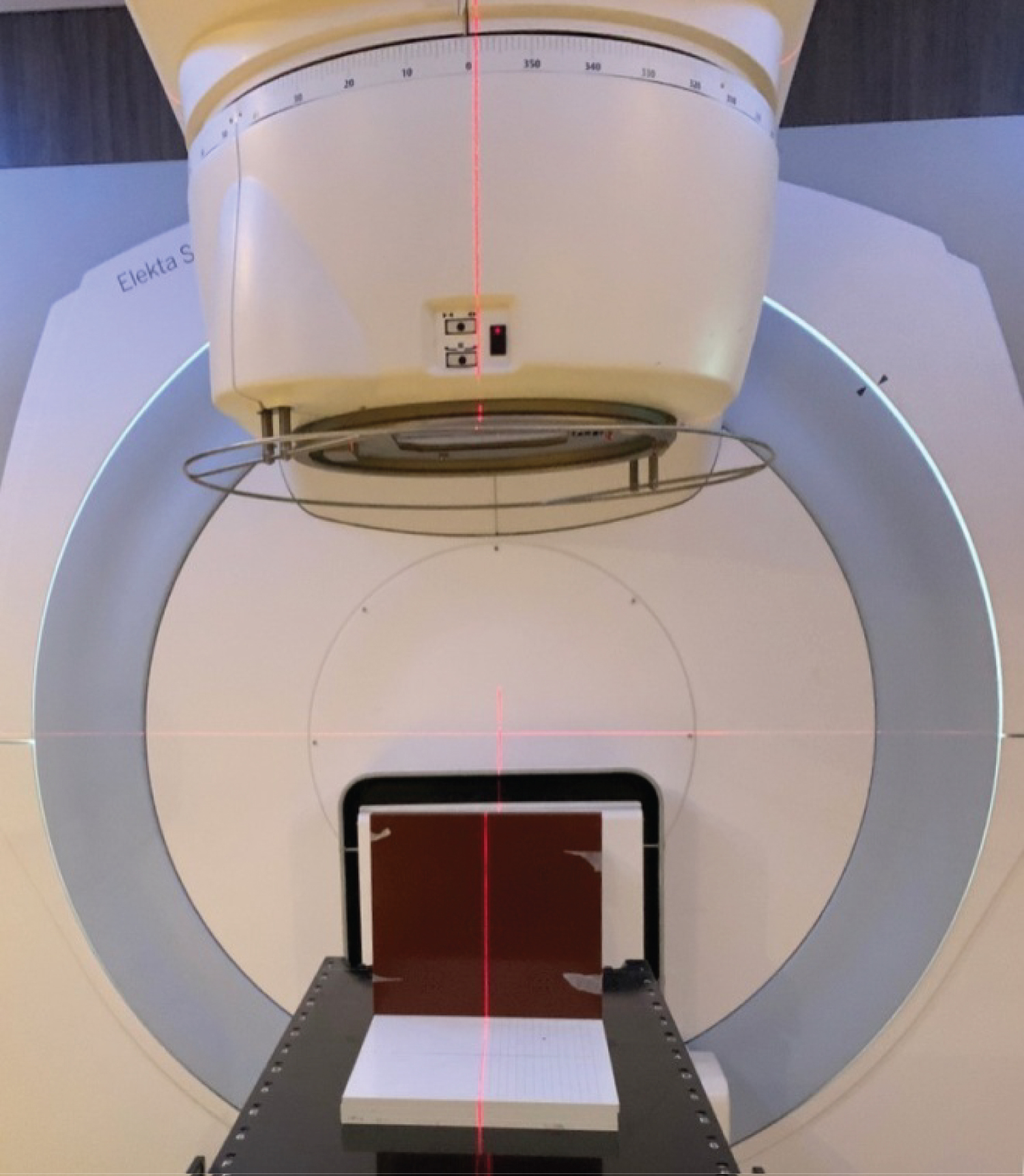 Figure 2: Elekta Linear Accelerator with Water Phantom Solid positioning in the gantry.
View Figure 2
Figure 2: Elekta Linear Accelerator with Water Phantom Solid positioning in the gantry.
View Figure 2
The solid water phantom used in the tests was built with solid water plates. It was used two plates of 30 × 30 × 1 cm3 and a complementary plate of 30 × 30 × 2 cm2. These plates responds to radiation beams similarly to water, with an error of 1% and helps in the search for data on dose distribution, as it approximates the absorption and dispersion properties of radiation from muscles and other soft tissues. This material allows better handling as it is solid and widely used in the manufacture of human phantoms [19,20].
Figure 3 shows two setups for positioning of the solid water phantom loaded with a film sheet. In the first setup, the phantom is irradiated laterally by the 10 MV photon beam, to record the absorbed dose variations in depth. For this setup the film sheet is loaded along the side edge of the phantom. In the second setup, the phantom is irradiated frontally, to record the dose variatons in the XY axial plane and the film sheet is placed in the center of the plate at a depth of 1.0 cm.
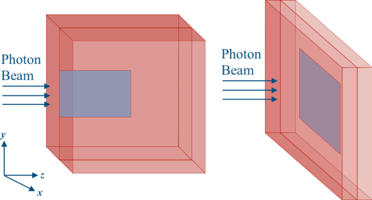 Figure 3: Solid water phantom setups loaded with a sheet of film for irradiation by the 10 MV photon beam, laterally and frontally.
View Figure 3
Figure 3: Solid water phantom setups loaded with a sheet of film for irradiation by the 10 MV photon beam, laterally and frontally.
View Figure 3
The film sheets used to record the dose profile were the GAFCHROMIC FILM, model EBT QD+, used in the experiments. This film has a construction characteristic similar to other models of radiochromic films, being a tool for a wide range of doses, equivalent to soft tissues, and can be handled in light rooms. The Gafchromic EBT Dosimetric Films is made by laminating a sensitive layer between two layers of polyester and it is used for measurements of absorbed doses in a range of 0.4 to 40 Gy and have a low dependence on beam energy, making it more suitable for applications in radiotherapy and radiosurgeries.
Radiochromic films when exposed to radiation show a darkening proportional to the dose received as higher is the absorbed dose, as darker they become. The film used has an active layer with 25 μm thickness. The calibration curves of the films are produced to allow the conversion of the darkening values into absorbed dose values. The film, after being irradiated, was stored in a place without humidity and away from sunlight, so that there was no interference in the chemical reactions of diacetylene compounds [21-24].
The Figure 4 shows two images of eight radiochomic film strips. These strips were irradiated with different doses. In Figure 4a is possible to observe the change of the strip colors. The first strip, the lightest, wasn't irradiated and the darkest strip is the highest recorded dose. The Figure 4b is the same image as the Figure 4a, after being worked on to separate the red channel image from the color image.
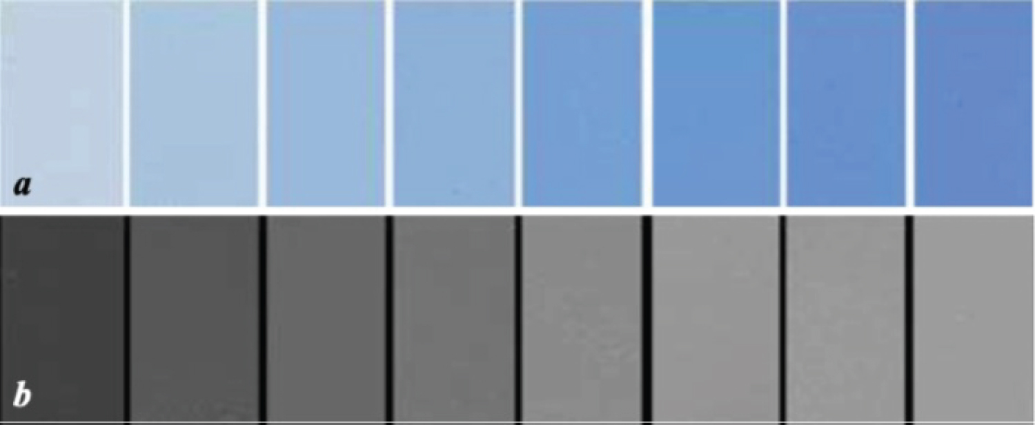 Figure 4: Images of film strips exposed in different absorbed dose values. Images after exposition (a) and images of the red channel after processing (b).
View Figure 4
Figure 4: Images of film strips exposed in different absorbed dose values. Images after exposition (a) and images of the red channel after processing (b).
View Figure 4
To record the absorbed dose profiles, the phantom loaded with a radiochromic film sheet was positioned in two different configurations (Figure 3), in order to obtain the axial and longitudinal absorbed dose variations, for each field size, when the phantom was irradiated with the photon beam of 10 MV.
In the assembly to obtain the longitudinal dose profiles, the film sheet was positioned between the two plates of solid water and it was irradiated laterally. In the irradiation to obtain the axial dose profiles, the film sheet was positioned inside the plates, in the center of the solid water phantom at a depth of 1.0 cm, being irradiated frontally.
The film sheets were cut for longitudinal and axial irradiations with specific sizes for each field size. Four lateral and four frontal irradiations were performed, one each for field size. The film sheets were cut according with the field size and the photon beam incidency, in the table (Table 1) have the sizes of the film sheets used.
Table 1: Film sheet sizes. View Table 1
After irradiation, the film sheets were left to rest for a minimum period of 24 h to stabilize of the reactions and the recorded image. Then, digital images were generated using a scanner device model Scanjet G4050 produced by HP. Digital images of the film sheets were acquired before the irradiation. The images were acquired at a resolution of 300 dpi with the suffix .tiff in color.
The digital images of the film sheets were processed in the imageJ software using the split tool to separate the Red, Blue and Green (RGB) color channels. In the Figure 5 are the images of the film sheets irradiated frontally and laterally, for the field of 5 × 5 cm2.
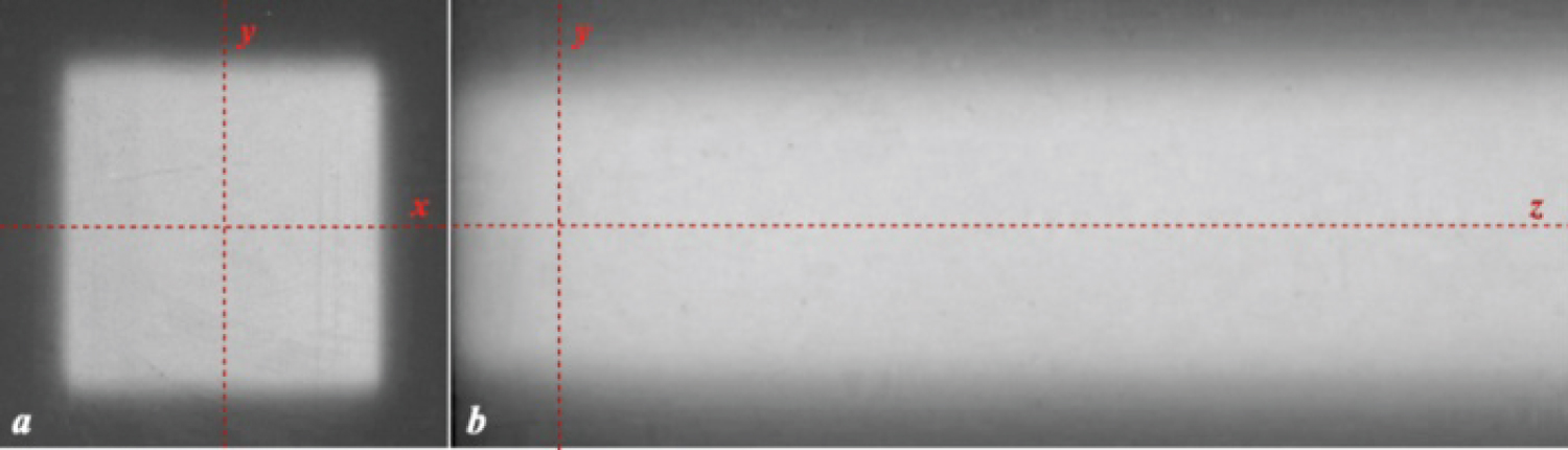 Figure 5: Irradiated radiochromic film sheets placed into the water phantom. color (a) and red channel images (b).
View Figure 5
Figure 5: Irradiated radiochromic film sheets placed into the water phantom. color (a) and red channel images (b).
View Figure 5
These images are of the red chanel component, separated by the split tool and with the grayscale inversion. Grayscale inversion is required to correlate the lightest color with the higest absorbed dose value. In these images are the positions of the axial (X and Y) and longitudinal Z axes, which were used to generate the absorbed dose profiles.
The image of the red color channel was chosen because the gray scale values in this channel are higher than those presented by the green and blue channels. The highest recorded dose value corresponds to the lightest register that appears in the film image worked on image J software. This will be the highest numerical value in grayscale.
Therefore, the red channel was chosen for the recording of absorbed doses, as it has the highest numerical value and a greater amplitude than the green and blue channels. The graph presented in Figure 6 contains the response curves related to the images of the three channels on the central longitudinal axis (Z).
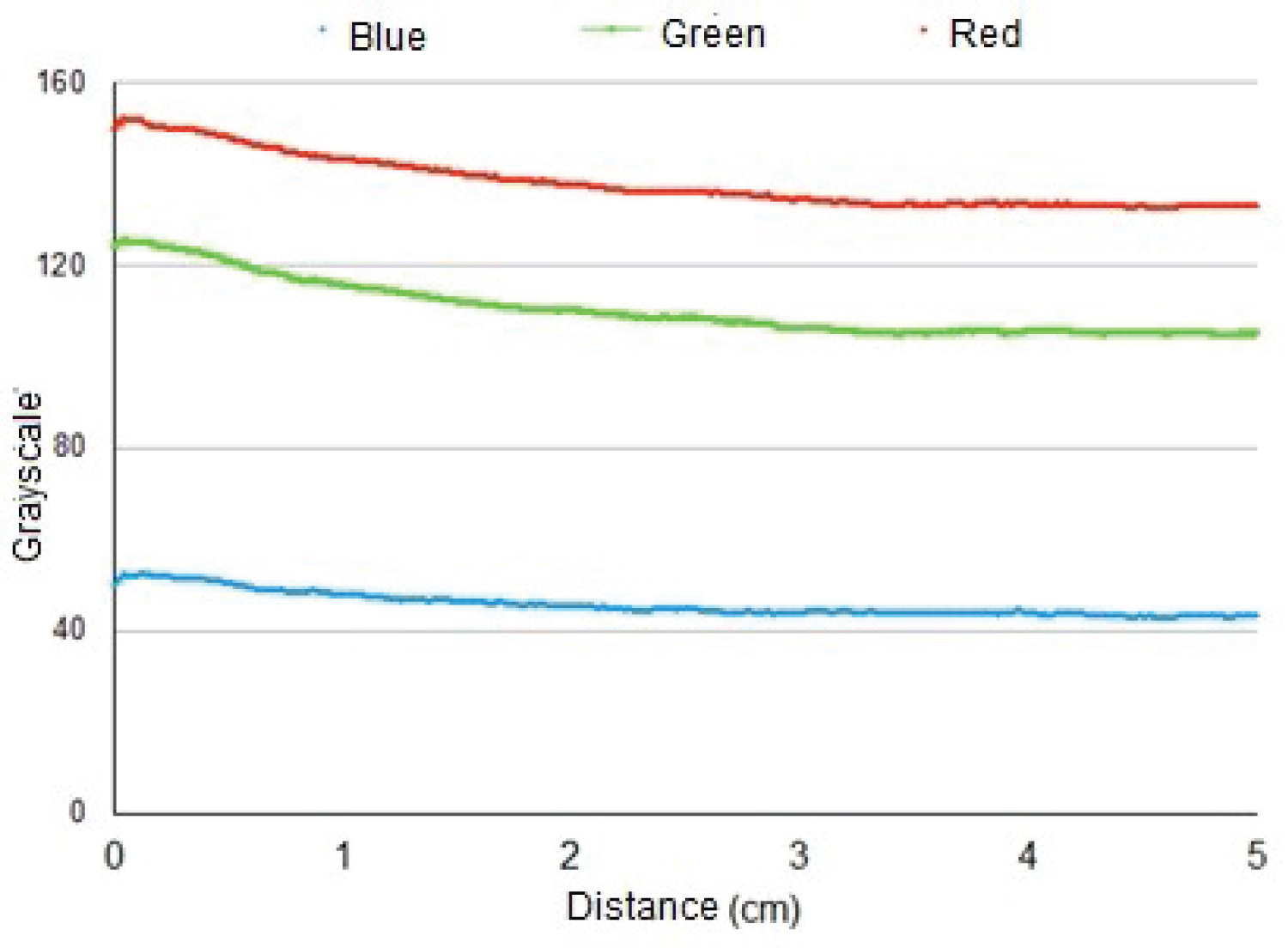 Figure 6: Intensity of the darkening response of an irradiated film strip, per RGB channel.
View Figure 6
Figure 6: Intensity of the darkening response of an irradiated film strip, per RGB channel.
View Figure 6
The solid water phantom was irradiated by a 10 MV photon beam. Irradiations were performed with the application of 300 monitor units (MU), which corresponds to a maximum absorbed dose of 2.97 Gy. Axial and longitudinal variations of the relative absorbed dose were obtained for the field sizes of 1 × 1 cm2, 2 × 2 cm2, 3 × 3 cm2 and 5 × 5 cm2, with the phantom surface placed at 1.0 m from the source.
The variations of the relative absorbed dose in depth are shown in Figure 7. The curves show the longitudinal variations for the four field sizes. The absorbed dose starts in zero and increases to the maximum value (peak). This graph shows the position where the film sheets were placed to acquire the axial curves in the XY plane, at a depth of 1 cm.
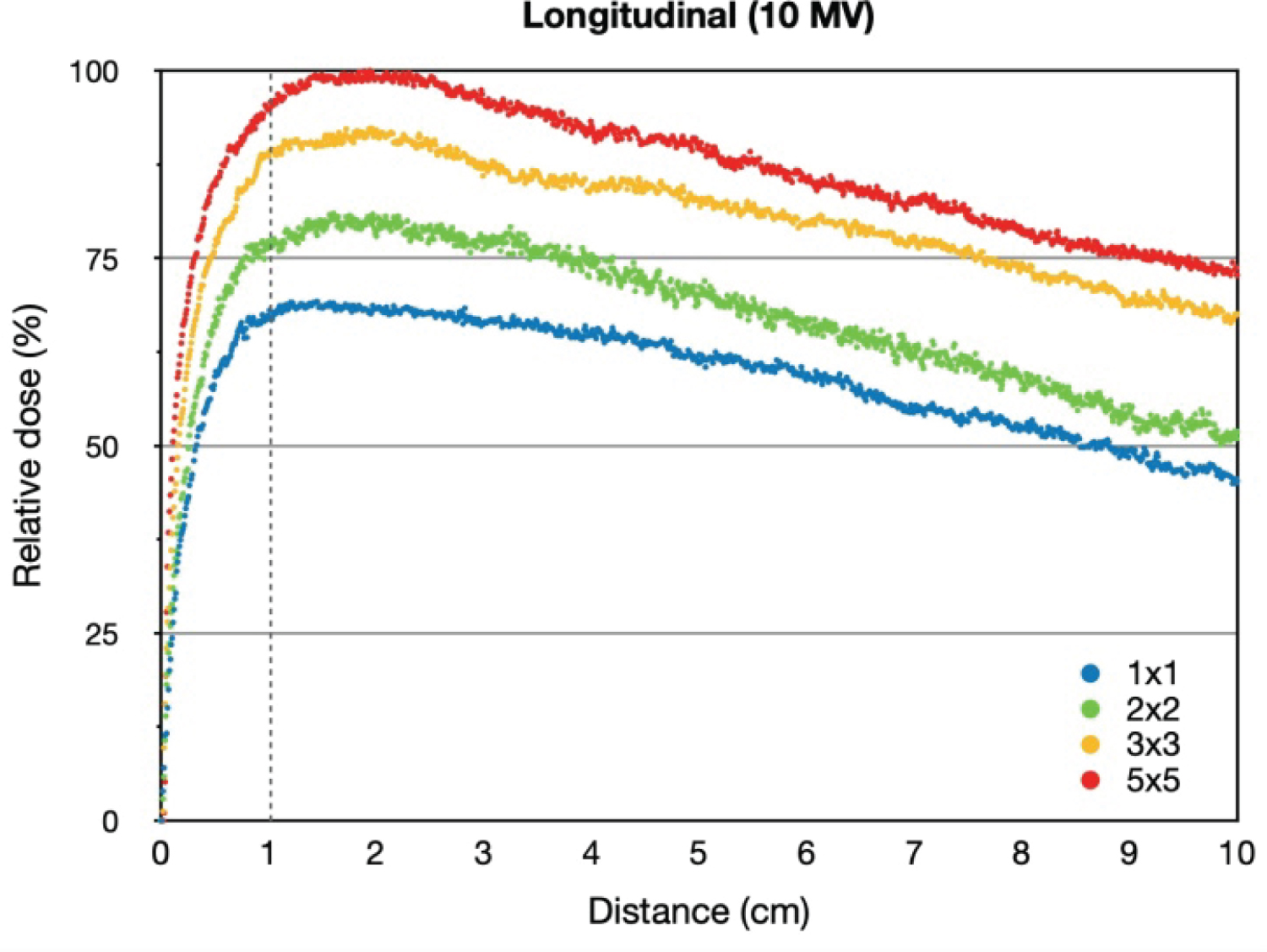 Figure 7: Relative absorbed dose variations at depth of different field sizes in the solid water phantom using a 10 MV photon beam.
View Figure 7
Figure 7: Relative absorbed dose variations at depth of different field sizes in the solid water phantom using a 10 MV photon beam.
View Figure 7
Considering the field sizes, the average peak value occurs at a distance of 1.89 ± 0.09 cm. At this point, the relative absorbed dose ranged from 100% for the 5 × 5 cm2 field to 69.23% for the 1 × 1 cm2 field. In all positions, the absorbed dose values were higher for the 5 × 5 cm2 field and lower for the smaller field sizes.
From the zero point to the distance of 1.89 cm the absorbed dose increase from zero to the maximum value (build-up region). After this point the values going decreasing with the deep.
At 1.0 cm depth, the relative absorbed dose varied from 95.16% to 67.28% for the fields of 5 × 5 cm2 and 1 × 1 cm2, respectively. At 10.0 cm depth, the variation of relative absorbed dose was from 73.70% to 45.27% for the fields of 5 × 5 cm2 and 1 × 1 cm2, respectively. The Table 2 presents results of relative absorbed dose of some points to the lateral irradiation of the solid water phantom.
Table 2: Relative absorbed dose values for longitudinal irradiation. View Table 2
Observing the longitudinal curves and comparing the values of Table 2, the dose values of the smaller fields were smaller across the observed distance. This reduction in the dose values is more expressive for the fields of 1 × 1 and 2 × 2 cm2. Considering the peak values, there was a dose reduction of 30.77%, 19.05% and 7.59%, for fields 1 × 1, 2 × 2 and 3 × 3 cm2, respectively.
Figure 8 shows the relative absorved dose variations for the frontal irradiation of the solid water phantom to the X axis, using field sizes of 1 × 1, 2 × 2, 3 × 3 and 5 × 5 cm2. These profiles were recorded at a depth of 1 cm in the phantom.
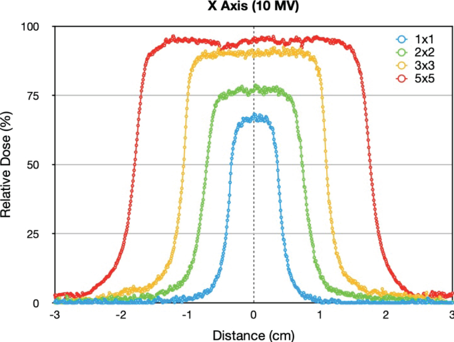 Figure 8: Relative absorbed dose variations for different field sizes measured on the X axis at 1 cm depth, in the solid water simulator irradiated with a 10 MV photon beam.
View Figure 8
Figure 8: Relative absorbed dose variations for different field sizes measured on the X axis at 1 cm depth, in the solid water simulator irradiated with a 10 MV photon beam.
View Figure 8
The curves have a plateau region where is the highest dose values. The average dose in the plateau regions varied from 93.87% to 65.90% for the field sizes of 5 × 5 and 1 × 1 cm2, respectively. The measurement point (1.0 cm) is in the build-up region, before the peak point (1.89 cm). Therefore, the recorded values are just below the values in the peak point.
Table 3 shows the average values of relative absorbed dose and standard deviation, for each field size. These values were selected considering the central area of the curves and the distance of the values used varied according to the plateau size. The maximum relative dose values found at these selected distances are displayed.
Table 3: Relative absorbed dose values in the plateau region for the X axis. View Table 3
The absorbed dose values in the plateaus were smaller for the smaller fields, with some oscillations in the plateau, mainly in the 5 × 5 cm2. The biggest absorbed dose reductions in this region happened in the two smaller fields of 1 × 1 and 2 × 2 cm2, about 29.80% and 20.09%, respectively.
Figure 9 shows the relative absorved dose variations in the frontal irradiation of the solid water phantom to the Y axis, using field sizes of 1 × 1, 2 × 2, 3 × 3 and 5 × 5 cm2. These profiles were recorded at a depth of 1 cm in the solid water phantom.
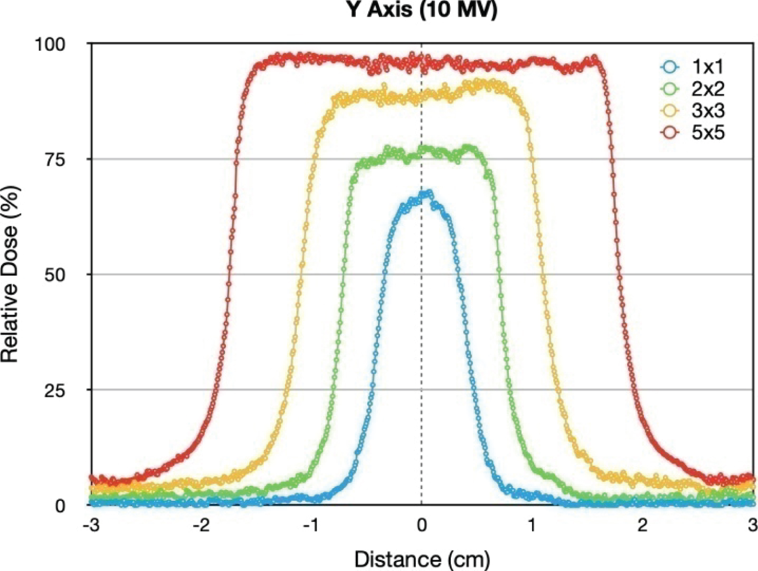 Figure 9: Relative absorbed dose variations for different field sizes measured on the Y axis at 1 cm depth, in the solid water simulator irradiated with a 10 MV photon beam.
View Figure 9
Figure 9: Relative absorbed dose variations for different field sizes measured on the Y axis at 1 cm depth, in the solid water simulator irradiated with a 10 MV photon beam.
View Figure 9
The average dose in plateau regions varied from 95.62% to 64.79% for the field sizes of 5 × 5 and 1 × 1 cm2, respectively. As the measurement point (1.0 cm) is before peak point (1.89 cm) and the recorded relative absorbed doses for each field size are just below the values in the peak point.
Table 4 shows the average values of relative absorbed dose and standard deviation, for each field size. The plateau size considered for the calculations varied from 3 to 0.5 cm according to the field size. The maximum relative dose values found for these selected distances are displayed. The maximum value of field 5 × 5 cm2 reached to 97.73% and smaller fields had smaller relative absorbed dose values.
Table 4: Relative absorbed dose values in the plateau region for the Y axis. View Table 4
Comparing the axial curves in the X and Y axes, they are similar, and the differences are greater for the field of 1 × 1 cm2 where, in the Y axis, the base is larger and the top more arrow, possibly caused by the influence of the position that these collimators are in relation to the photon source.
The isodose curves are used to represent the absorbed dose variations in a plane. The absorbed dose distribution is represented by curves generated by points where the dose values are equal. Isodose curves are regular absorbed dose intervals drawn as depth dose distribution maps and can be expressed as a percentage of the absorbed dose at a reference point [2,18,25].
The Figure 10 shows isodose curves for the field sizes of 1 × 1, 2 × 2, 3 × 3 and 5 × 5 cm2 measured at 1 cm depth in the frontal irradiation of the solid water phantom. The film area shown in the figure for each field size is 6 × 6 cm2. In these curves it is possible to observe the square characteristic of the field shape and the differences in the size of the irradiated area.
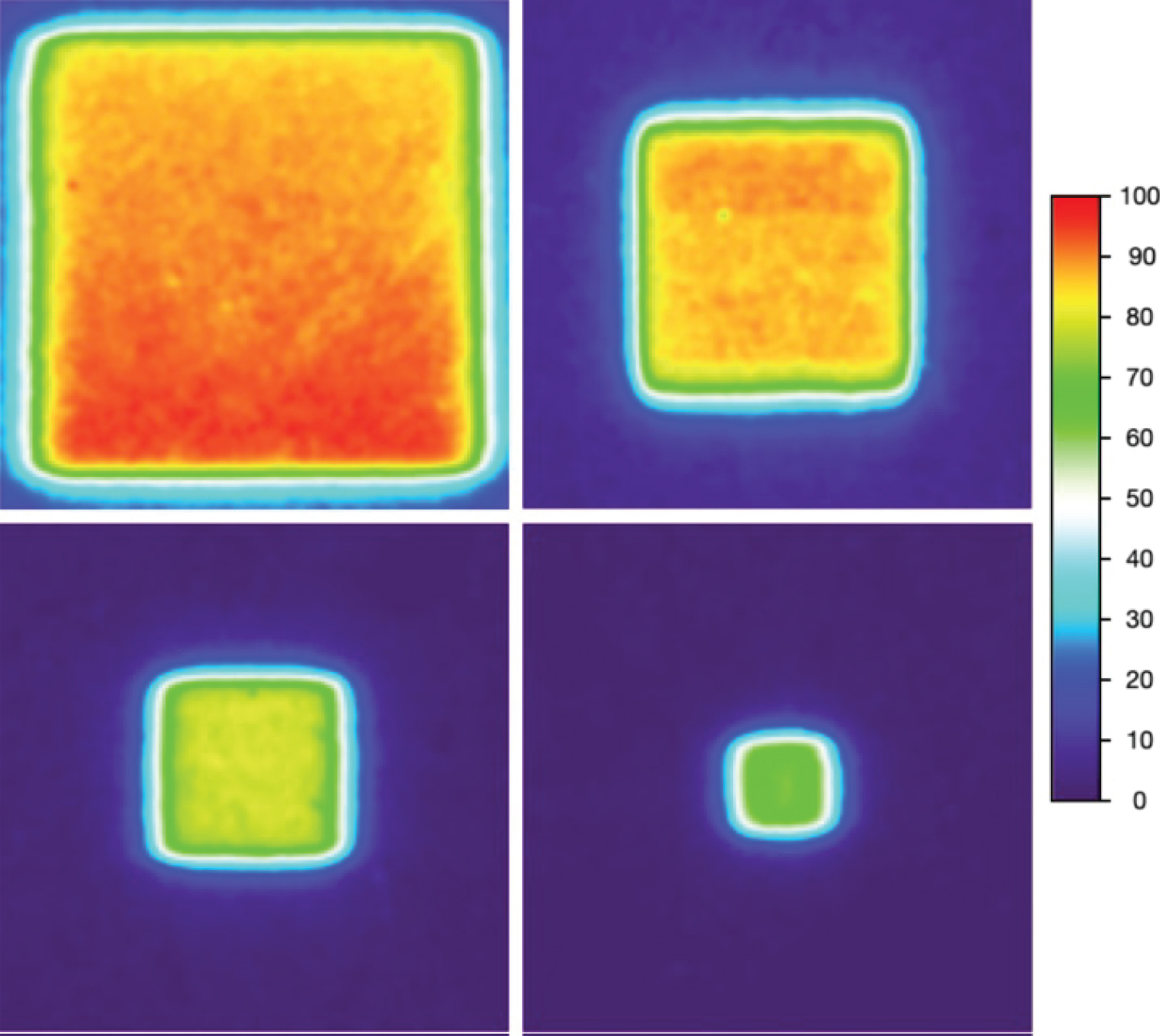 Figure 10: Isodose curves at 1.0 cm deep for fields 1 × 1, 2 × 2, 3 × 3 and 5 × 5 cm2 in a Solid Water Phantom using 10 MV photon beam.
View Figure 10
Figure 10: Isodose curves at 1.0 cm deep for fields 1 × 1, 2 × 2, 3 × 3 and 5 × 5 cm2 in a Solid Water Phantom using 10 MV photon beam.
View Figure 10
The color scale starts in dark blue and ends in red, corresponding to the variation of the relative absorbed dose from zero to 100% in this XY plane, which is 1 cm deep. It should be noted that the maximum dose that occurs in this plane corresponds to 97.3% of the peak dose (100%) that occurs in the 5 × 5 field size. The maximum absorbed dose occurs at a deeper region of the solid water phantom.
In the central area of the images, absorbed doses close to the maximum dose in this XY plane (100%) are recorded in red and orange, for field sizes of 5 × 5 and 3 × 3 cm2. In the 2 × 2 cm2 field size, the central region is colored yellow, corresponding to absorved doses close to 80% of the maximum absorbed dose in this plane XY and in the 1 × 1 cm2 field size the central region is colored green, corresponding to doses close to 65% of the maximum absorbed dose in this plane, according to the color scale variations.
Comparing the isodose curves with the axial curves, it's possible to observe the variation found in the axial curves of the X and Y axes occurs in the isodose curves. In these curves it is possible to observe the entire the dose distribution in the axial plane XY and the irradiation field limits.
In this work, a solid water phantom was irradiated by a photom beam generated with a 10 MV voltage from a Linear Accelerator. The phantom was irradiated in four different field sizes, including small field sizes. The water phantom was irradiated with 3 MU, corresponding to 2.97 Gy in the maximum dose value.
Absorved dose measurements were performed using radiochromic film sheets inside the solid water phantom. These films recorded the absorbed dose variation profile in depth and in a specific axial plane at 1 cm depth.
It was observed variations in the behaviour of the dose deposition in depth, where all the values of the small fields were smaller. As smaller was the field size, as smaller was the absorved dose.